library(tidyverse)
theme_set(theme_bw())
library(yspec)
library(mrgsolve)
library(mrggsave)
library(vpc)
library(glue)
library(bbr)
library(here)1 Introduction
This document illustrates the mechanics of using the vpc package along with mrgsolve to create Visual Predictive Check plots.
2 Tools used
2.1 MetrumRG packages
mrgsolve Simulate from ODE-based population PK/PD and QSP models in R.
yspec Data specification, wrangling, and documentation for pharmacometrics.
bbr Manage, track, and report modeling activities, through simple R objects, with a user-friendly interface between R and NONMEM®.
mrggsave Label, arrange, and save annotated plots and figures.
2.2 CRAN packages
vpc Create visual predictive checks.
3 Outline
- First the we load the analysis data set that was used in the NONMEM® estimation
- Next, we’ll load an mrgsolve translation of the NONMEM® model and validate the coding against outputs from the NONMEM® run
- After simulating data replicates from the mrgsolve model, we’ll construct four visual predictive checks
- Basic VPC on dose-normalized concentrations
- VPC for a single dose, stratified by a covariate
- VPC on fraction below the quantitative limit versus
- Prediction-corrected VPC
4 Required packages
All packages were installed from mpn via pkgr.
These are some global options which reflect the directory structure associated with this project
options(mrggsave.dir = tempdir(), mrg.script = "pk-vpc-final.Rmd")
options(mrgsolve.project = here("script/model"))
This is a theme that we’ll use to style the plots coming out of vpc.
mrg_vpc_theme = new_vpc_theme(list(
  sim_pi_fill = "steelblue3", sim_pi_alpha = 0.5,
  sim_median_fill = "grey60", sim_median_alpha = 0.5
))
5 Setup
5.1 Data
First, we have some observations that are below the limit of quantification that need to be dealt with.
The final model estimation run was 106, so we read back those results using bbr::nm_join(). You can read more about using bbr for model management here Model Management.
runno <- 106
data <- nm_join(here("model/pk/106"), .superset = TRUE)
We want to load in the complete data, including observations that were ignored in the estimation run because they were below the quantitation limit (BQL). To do this, we pass .superset = TRUE to nm_join(). The result is the full model estimation data set along with all items that were tabled from that run. Be sure to also drop any rows that were excluded from the model estimation run for reasons other than being below the quantitation limit.
data <- filter(data, is.na(C))

head(data)
# A tibble: 6 × 49
C NUM ID TIME SEQ CMT EVID AMT DV.DATA AGE WT HT
<lgl> <dbl> <int> <dbl> <int> <int> <int> <int> <dbl> <dbl> <dbl> <dbl>
1 NA 1 1 0 0 1 1 5 0 28.0 55.2 160.
2 NA 2 1 0.61 1 2 0 NA 61.0 28.0 55.2 160.
3 NA 3 1 1.15 1 2 0 NA 91.0 28.0 55.2 160.
4 NA 4 1 1.73 1 2 0 NA 122. 28.0 55.2 160.
5 NA 5 1 2.15 1 2 0 NA 126. 28.0 55.2 160.
6 NA 6 1 3.19 1 2 0 NA 84.7 28.0 55.2 160.
# ℹ 37 more variables: EGFR <dbl>, ALB <dbl>, BMI <dbl>, SEX <int>, AAG <dbl>,
# SCR <dbl>, AST <dbl>, ALT <dbl>, CP <int>, TAFD <dbl>, TAD <dbl>,
# LDOS <int>, MDV <int>, BLQ <int>, PHASE <int>, STUDYN <int>, DOSE <int>,
# SUBJ <int>, USUBJID <chr>, STUDY <chr>, ACTARM <chr>, RF <chr>,
# IPRED <dbl>, NPDE <dbl>, CWRES <dbl>, CL <dbl>, V2 <dbl>, Q <dbl>,
# V3 <dbl>, KA <dbl>, ETA1 <dbl>, ETA2 <dbl>, ETA3 <dbl>, DV <dbl>,
# PRED <dbl>, RES <dbl>, WRES <dbl>We will use the data specification object that corresponds with the model estimation data (in this case pk)
spec <- ys_load(here("data/derived/pk.yml"))
spec <- ys_namespace(spec, "long")
The function ys_get_short_unit() will pull the “short” name from each column name and append the unit if available
lab <- ys_get_short_unit(spec, parens = TRUE, title_case = TRUE)The function ys_add_factors() will look at spec for discrete data items and append them to the data set as factors
data <- ys_add_factors(data, spec)For example
count(data, CP, CP_f)# A tibble: 4 × 3
CP CP_f n
<int> <fct> <int>
1 0 CP score: 0 3880
2 1 CP score: 1 160
3 2 CP score: 2 160
4 3 CP score: 3 160For convenience we will set aliases for a couple of these columns
data <- mutate(data, Hepatic = CP_f, Renal = RF_f)5.2 The simulation model
This should reflect the nonmem model model/pk/106.ctl
mod <- mread(glue("{runno}.mod"))5.2.1 Validate simulation model
We can validate our coding of the model, looking at PRED returned from NONMEM® as compared to PRED returned from simulation from the model.
We already have PRED in the data
select(data, ID, TIME, DV, IPRED, PRED)# A tibble: 4,360 × 5
ID TIME DV IPRED PRED
<int> <dbl> <dbl> <dbl> <dbl>
1 1 0 0 0 0
2 1 0.61 61.0 68.5 60.6
3 1 1.15 91.0 90.8 78.5
4 1 1.73 122. 97.3 83.0
5 1 2.15 126. 96.7 82.2
6 1 3.19 84.7 88.7 75.5
7 1 4.21 62.1 78.9 67.8
8 1 5.09 49.1 71.1 61.7
9 1 6.22 64.2 62.4 54.8
10 1 8.09 59.6 51.0 45.7
# ℹ 4,350 more rowsWe’ll modify the mrgsolve model object to return PRED when we simulate
pmod <- zero_re(mod)

check <- mrgsim(pmod, data = data, recover = "PRED,EVID", digits = 5)

head(check) %>% select(ID, TIME, Y, PRED)
ID TIME Y PRED
1 1 0.00 0.000 0.000
2 1 0.61 60.580 60.580
3 1 1.15 78.543 78.543
4 1 1.73 83.035 83.035
5 1 2.15 82.217 82.217
6 1 3.19 75.482 75.482Keeping only observations
check <- filter(check, EVID==0)we do a quick summary and show that all 3210 PRED values are matching between the mrgsolve model and NONMEM® output
nrow(check) [1] 3210summary(check$Y - check$PRED) Min. 1st Qu. Median Mean 3rd Qu. Max. NA's
0 0 0 0 0 0 68 This demonstrates that the simulation model can reproduce the population predictions from the estimation model and is reliable for use to simulate the predictive check.
6 VPC on dose-normalized concentrations
In this example, we will normalize the observed and simulated data from SAD and MAD studies (Studies 1 and 2) and present all doses in the same plot.
Studies 1 and 2 were single- and multiple-ascending dose studies with healthy volunteers
count(data, STUDY, STUDYN, CP_f, RF_f)# A tibble: 10 × 5
STUDY STUDYN CP_f RF_f n
<chr> <int> <fct> <fct> <int>
1 101-DEMO-001 1 CP score: 0 No impairment 480
2 101-DEMO-002 2 CP score: 0 No impairment 1800
3 201-DEMO-003 3 CP score: 0 No impairment 360
4 201-DEMO-003 3 CP score: 0 Mild impairment 360
5 201-DEMO-003 3 CP score: 0 Moderate impairment 360
6 201-DEMO-003 3 CP score: 0 Severe impairment 360
7 201-DEMO-004 4 CP score: 0 No impairment 160
8 201-DEMO-004 4 CP score: 1 No impairment 160
9 201-DEMO-004 4 CP score: 2 No impairment 160
10 201-DEMO-004 4 CP score: 3 No impairment 160sad_mad <- filter(data, STUDYN <= 2)6.1 The simulation function
Create a function to simulate out one replicate and re-use it for all the different simulations we will use for the predictive checks.
sim <- function(rep, data, model,
                recover = "EVID,DOSE,STUDY,Renal,Hepatic") {
  mrgsim(
    model,
    data = data,
    carry_out = "NUM",
    recover = recover,
    Req = "Y",
    output = "df"
  ) %>%  mutate(irep = rep)
}
Arguments
repthe current replicate numberdatathe data template for simulationmodelthe mrgsolve model objectrecovercolumns to carry from the data into the output
Return
A data frame with the replicate number appended as irep.
6.2 Simulate for VPC
We’ll simulate only 100 replicates here to save some computation time; we would typically simulate more in a production context.
isim <- seq(100)

set.seed(86486)

sims <- lapply(
  isim, sim,
  data = sad_mad,
  mod = mod
) %>% bind_rows()
Filter both the observed and simulated data on
- actual observations that are not BQL
- simulated observations that are above the limit of quantitation (here 10 ng/mL)
fsad_mad <-  filter(sad_mad,  EVID==0, BLQ ==0)
fsims <- filter(sims, EVID==0, Y >= 10)
Also we are going to dose-normalize observed and simulated data so we can put all the doses on the same plot
fsad_mad <-  mutate(fsad_mad,  DVN = DV/DOSE)
fsims <- mutate(fsims, YN = Y/DOSE)
6.3 Calculate VPC and plot
Pass observed and simulated data into vpc() function, noting that we want this stratified by STUDY so that SAD and MAD regimens are plotted separately
p1 <- vpc(
  obs = fsad_mad,
  sim = fsims,
  stratify = "STUDY",
  obs_cols = list(dv = "DVN"),
  sim_cols=list(dv = "YN", sim = "irep"),
  log_y = TRUE,
  pi = c(0.05, 0.95),
  ci = c(0.025, 0.975),
  facet = "columns",
  show = list(obs_dv = TRUE),
  vpc_theme = mrg_vpc_theme
)
Notes
- We want this vpc to show dose-normalized concentrations, so we change the name of
dvunderobs_colsandsim_cols - Setting
pitoc(0.05, 0.95)indicates that the vpc will show the 5th and 95th percentiles of observed and simulated data in addition to the median - Setting
citoc(0.025, 0.975)indicates that we want to display 95% prediction intervals around the simulated statistics (median, 5th and 95th percentiles - The
showargument indicates that we want observed data points on the plot
p1 <-
  p1 +
  xlab(lab$TIME) +
  ylab("Dose-normalized concentration (ng/mL)")

p1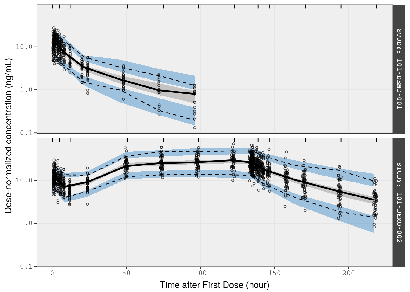
mrggsave_last(stem = "pk-vpc-{runno}-dose-norm", height = 7.5)7 VPC stratified on a covariate
In this example, we’ll take a subset of the data from the renal study (Study 3) and stratify the VPC on the Renal Function covariate
rf_data <- filter(data, STUDYN==3) set.seed(54321)
rf_sims <- lapply(
isim, sim,
data = rf_data,
mod = mod
) %>% bind_rows()Filtering both the observed and simulated data; there was only a single dose administered in this study
f_rf_data <- filter(rf_data, EVID==0, BLQ ==0)
f_rf_sims <- filter(rf_sims, EVID==0, Y >= 10)
Calculate the vpc and plot
p2 <- vpc(
  obs = f_rf_data,
  sim = f_rf_sims,
  stratify = "Renal",
  obs_cols = list(dv = "DV"),
  sim_cols=list(dv = "Y", sim = "irep"),
  log_y = TRUE,
  pi = c(0.05, 0.95),
  ci = c(0.025, 0.975),
  show = list(obs_dv = TRUE),
  vpc_theme = mrg_vpc_theme
)

p2 <- p2 +  xlab(lab$TIME) + ylab("Concentration (ng/mL)")

p2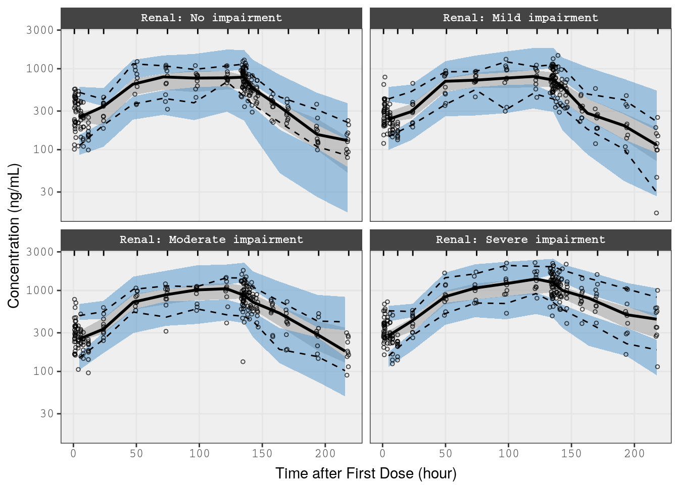
mrggsave_last(stem = "pk-vpc-{runno}-rf", height = 6.5)We can also run vpc stratified on hepatic function
Show the code
cp_data <- filter(data, STUDYN==4)

set.seed(7456874)

cp_sims <- lapply(
  isim,
  sim,
  data = cp_data,
  mod = mod
) %>% bind_rows()

f_cp_data <- filter(cp_data, EVID==0, BLQ ==0)
f_cp_sims <- filter(cp_sims, EVID==0, Y >= 10)

p3 <- vpc(
  obs = f_cp_data,
  sim = f_cp_sims,
  stratify = "Hepatic",
  obs_cols = list(dv = "DV"),
  sim_cols=list(dv="Y", sim="irep"),
  log_y = TRUE,
  pi = c(0.05, 0.95),
  ci = c(0.025, 0.975),
  labeller = label_value,
  show = list(obs_dv = TRUE),
  vpc_theme = mrg_vpc_theme
)

p3 <-
  p3 +
  xlab(lab$TIME) +
  ylab("Concentration (ng/mL)")

p3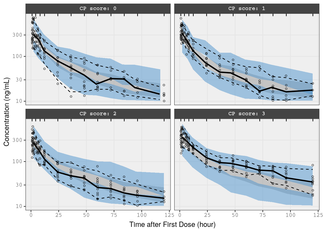
mrggsave(p3, stem = "pk-vpc-{runno}-cp", height = 6.5)8 VPC on fraction BLQ
This is a predictive check on the fraction of observations that are below the limit of quantification versus time. We’ll take just the single dose studies and limit the analysis out to 100 hours after the dose
data <- nm_join(here("model/pk/106"), .superset = TRUE)
data <- arrange(data, NUM)
data <- filter(data, STUDYN %in% c(1,3), TIME <= 100)
Simulate using the sim() function as we have done before
set.seed(7456874)

b_sims <- lapply(
  isim,
  sim,
  data = data,
  mod = mod
) %>% bind_rows()
Now, we use the vpc_cens() function from the vpc package and pass in the lower limit of quantification (lloq)
p4 <- vpc_cens(
  sim = b_sims,
  obs = data,
  lloq = 10,
  obs_cols = list(dv = "DV"),
  sim_cols = list(dv = "Y", sim = "irep")
)

p4 <- p4 + xlab(lab$TIME)

p4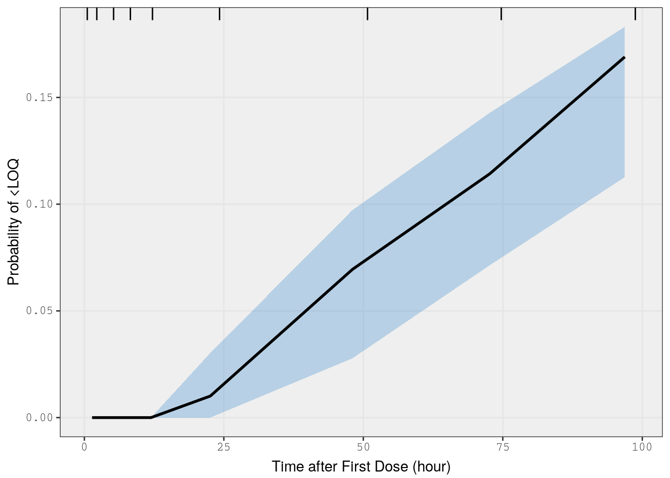
mrggsave_last(stem = "pk-vpc-{runno}-BLQ", height = 6.5)9 Prediction-corrected VPC
This VPC method removes variability in a time bin by “correcting” (or normalizing) observed and simulated data with the population predicted value (PRED). Recall that we used bbr::nm_join() to read in the analysis data set along with all the table output joined on. We’ll filter out the rows that were commented going into the analysis, but retain the rows that were ignored because they were BQL.
data <- nm_join(here("model/pk/106"), .superset = TRUE)
data <- filter(data, is.na(C))
This data set includes PRED as generated by NONMEM, but we don’t have those values for rows where the observations were BQL. We’ll use mrgsolve to simulate PRED for every row in the complete data set.
out <- mrgsim(zero_re(mod), data)Then, we’ll copy that value into the simulation data set for use in the prediction-corrected VPC. We’ll save the NONMEM version just as a check that the simulation went as planned.
data <- mutate(data, NMPRED = PRED, PRED = out$Y)

select(data, ID, TIME, DV, PRED, NMPRED, IPRED)
# A tibble: 4,360 × 6
ID TIME DV PRED NMPRED IPRED
<int> <dbl> <dbl> <dbl> <dbl> <dbl>
1 1 0 0 0 0 0
2 1 0.61 61.0 60.6 60.6 68.5
3 1 1.15 91.0 78.5 78.5 90.8
4 1 1.73 122. 83.0 83.0 97.3
5 1 2.15 126. 82.2 82.2 96.7
6 1 3.19 84.7 75.5 75.5 88.7
7 1 4.21 62.1 67.8 67.8 78.9
8 1 5.09 49.1 61.7 61.7 71.1
9 1 6.22 64.2 54.8 54.8 62.4
10 1 8.09 59.6 45.7 45.7 51.0
# ℹ 4,350 more rowsTaking just single dose studies (1 and 4)
single <- filter(data, STUDYN %in% c(1,4))out <- lapply(
seq(200),
FUN = sim,
data = single,
model = mod,
recover = "PRED,DV,EVID,DOSE"
) %>% bind_rows()Get simulated and observed data ready so that PRED is in both the simulated and observed data
observed <- filter(single, EVID==0, BLQ==0)
simulated <- filter(out,   EVID==0, Y >= 10)

head(simulated)
ID TIME NUM Y PRED DV EVID DOSE irep
1 1 0.61 2 44.44512 60.57972 61.005 0 5 1
2 1 1.15 3 31.71695 78.54283 90.976 0 5 1
3 1 1.73 4 59.28731 83.03472 122.210 0 5 1
4 1 2.15 5 66.51486 82.21690 126.090 0 5 1
5 1 3.19 6 80.44592 75.48245 84.682 0 5 1
6 1 4.21 7 55.79783 67.79305 62.131 0 5 1head(observed)# A tibble: 6 × 50
C NUM ID TIME SEQ CMT EVID AMT DV.DATA AGE WT HT
<lgl> <dbl> <int> <dbl> <int> <int> <int> <int> <dbl> <dbl> <dbl> <dbl>
1 NA 2 1 0.61 1 2 0 NA 61.0 28.0 55.2 160.
2 NA 3 1 1.15 1 2 0 NA 91.0 28.0 55.2 160.
3 NA 4 1 1.73 1 2 0 NA 122. 28.0 55.2 160.
4 NA 5 1 2.15 1 2 0 NA 126. 28.0 55.2 160.
5 NA 6 1 3.19 1 2 0 NA 84.7 28.0 55.2 160.
6 NA 7 1 4.21 1 2 0 NA 62.1 28.0 55.2 160.
# ℹ 38 more variables: EGFR <dbl>, ALB <dbl>, BMI <dbl>, SEX <int>, AAG <dbl>,
# SCR <dbl>, AST <dbl>, ALT <dbl>, CP <int>, TAFD <dbl>, TAD <dbl>,
# LDOS <int>, MDV <int>, BLQ <int>, PHASE <int>, STUDYN <int>, DOSE <int>,
# SUBJ <int>, USUBJID <chr>, STUDY <chr>, ACTARM <chr>, RF <chr>,
# IPRED <dbl>, NPDE <dbl>, CWRES <dbl>, CL <dbl>, V2 <dbl>, Q <dbl>,
# V3 <dbl>, KA <dbl>, ETA1 <dbl>, ETA2 <dbl>, ETA3 <dbl>, DV <dbl>,
# PRED <dbl>, RES <dbl>, WRES <dbl>, NMPRED <dbl>Now in the vpc() call, we can just set pred_corr = TRUE
p5 <- vpc(
  obs = observed,
  sim = simulated,
  obs_cols = list(dv = "DV"),
  sim_cols = list(dv = "Y", sim = "irep"),
  log_y = TRUE,
  pred_corr = TRUE,
  pi = c(0.05, 0.95),
  ci = c(0.025, 0.975),
  labeller = label_value,
  show = list(obs_dv = TRUE),
  vpc_theme = mrg_vpc_theme
)
p5 <-
p5 +
xlab(lab$TIME) +
ylab("Pred-corrected concentration (ng/mL)")
p5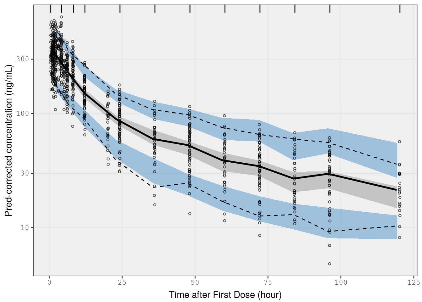
mrggsave_last(stem = "pk-vpc-{runno}-pc", height = 6.5)