library(here)
library(mrgsolve)
library(dplyr)
library(tidyr)
library(bbr)
library(pmtables)
library(data.table)
library(yspec)
library(mrgmisc)1 Introduction
This document provides an example of how mrgsolve can be used to simulate subject-specific exposures from empirical Bayes estimates (EBE) generated from a NONMEM estimation run. We will simulate exposures at each individual’s nominal dose and summarize by DOSE and renal function group.
2 Tools used
2.1 MetrumRG packages
mrgsolve Simulate from ODE-based population PK/PD and QSP models in R.
yspec Data specification, wrangling, and documentation for pharmacometrics.
pmtables Create summary tables commonly used in pharmacometrics and turn any R table into a highly customized tex table.
bbr Manage, track, and report modeling activities, through simple R objects, with a user-friendly interface between R and NONMEM®.
2.2 CRAN packages
dplyr A grammar of data manipulation.
3 Outline
First, we’ll prepare a model and data set for simulating subject-specific PK profiles from EBEs output from NONMEM®.
After simulating the data, we’ll create two summaries:
The first summary will look at exposures in subjects with normal renal function. We’ll create a table summarizing
Cmax,CminandAUCat steady state by dose.The second summary will look at steady state exposures across doses and renal function groups (e.g. mild, moderate, or severe renal impairment)
The summaries will be saved in table format to include in the report.
Finally, we’ll demonstrate how to preview tables in an environment that mimics our report formatting.
4 Required packages and options
These options are set to direct outputs.
options(
  mrgsolve.soloc = here("script/build"),
  bbr.verbose = FALSE,
  pmtables.dir = here("deliv/table")
)
We load the yspec object, which will provide information about the data set
spec <- ys_load(here("data/derived/pk.yml"))5 EBE simulation model
The final model run (model/pk/106) was a standard two-compartment model with first-order absorption. This means that we can simply use a model out of the internal library that ships with mrgsolve
mod <- modlib("pk2")This model is parameterized with CL, Vn, Q and KA
param(mod)
 Model parameters (N=5):
 name value . name value
 CL   1     | V2   20
 KA   1     | V3   10
 Q    2     | .    .
6 EBE simulation data set
Our strategy is to read in the output from run 106 where we tabled all of the subject-level EBEs and create a data set that will allow us to generate exposures using those parameter estimates.
We use nm_join() to get an integrated data frame of input and output data
data <- nm_join(here("model/pk/106"))
head(data)
# A tibble: 6 × 49
C NUM ID TIME SEQ CMT EVID AMT DV.DATA AGE WT HT
<lgl> <dbl> <int> <dbl> <int> <int> <int> <int> <dbl> <dbl> <dbl> <dbl>
1 NA 1 1 0 0 1 1 5 0 28.0 55.2 160.
2 NA 2 1 0.61 1 2 0 NA 61.0 28.0 55.2 160.
3 NA 3 1 1.15 1 2 0 NA 91.0 28.0 55.2 160.
4 NA 4 1 1.73 1 2 0 NA 122. 28.0 55.2 160.
5 NA 5 1 2.15 1 2 0 NA 126. 28.0 55.2 160.
6 NA 6 1 3.19 1 2 0 NA 84.7 28.0 55.2 160.
# ℹ 37 more variables: EGFR <dbl>, ALB <dbl>, BMI <dbl>, SEX <int>, AAG <dbl>,
# SCR <dbl>, AST <dbl>, ALT <dbl>, CP <int>, TAFD <dbl>, TAD <dbl>,
# LDOS <int>, MDV <int>, BLQ <int>, PHASE <int>, STUDYN <int>, DOSE <int>,
# SUBJ <int>, USUBJID <chr>, STUDY <chr>, ACTARM <chr>, RF <chr>,
# IPRED <dbl>, NPDE <dbl>, CWRES <dbl>, CL <dbl>, V2 <dbl>, Q <dbl>,
# V3 <dbl>, KA <dbl>, ETA1 <dbl>, ETA2 <dbl>, ETA3 <dbl>, DV <dbl>,
# PRED <dbl>, RES <dbl>, WRES <dbl>Next, we’ll subset that data frame down to doses
dose_rec <- filter(data, EVID==1)and then generate a data frame of subject-level parameters
pars <- distinct(
  dose_rec,
  ID, CL, V2, Q, V3, KA,
  AMT, RF, ACTARM, DOSE
)

head(pars)
# A tibble: 6 × 10
ID CL V2 Q V3 KA AMT RF ACTARM DOSE
<int> <dbl> <dbl> <dbl> <dbl> <dbl> <int> <chr> <chr> <int>
1 1 2.62 39.8 3.02 53.0 1.39 5 norm DEMO 5 mg 5
2 2 1.88 34.2 2.88 49.8 1.77 5 norm DEMO 5 mg 5
3 3 3.27 50.9 3.01 52.7 1.41 5 norm DEMO 5 mg 5
4 4 7.34 129. 4.10 79.7 3.38 5 norm DEMO 5 mg 5
5 5 6.75 133. 4.62 93.5 2.91 5 norm DEMO 5 mg 5
6 6 3.69 62.2 3.61 67.3 1.46 10 norm DEMO 10 mg 10This simulation is going to depend on the fact that our EBE parameter names (e.g. CL and V3) match up with the names of the parameters in the pk2 model from the internal library.
mrgsolve comes with a function to check names in the data against names in the model to help confirm that the two match up
inventory(mod, pars)Found all required parameters in 'pars'.Great! We have accounted for all the model names in our data set.
We’ll simulate exposures at steady state for once-daily dosing
dose <- mutate(pars, II = 24, SS = 1, TIME = 0, EVID = 1, CMT = 1)

head(dose)
# A tibble: 6 × 15
ID CL V2 Q V3 KA AMT RF ACTARM DOSE II SS TIME
<int> <dbl> <dbl> <dbl> <dbl> <dbl> <int> <chr> <chr> <int> <dbl> <dbl> <dbl>
1 1 2.62 39.8 3.02 53.0 1.39 5 norm DEMO … 5 24 1 0
2 2 1.88 34.2 2.88 49.8 1.77 5 norm DEMO … 5 24 1 0
3 3 3.27 50.9 3.01 52.7 1.41 5 norm DEMO … 5 24 1 0
4 4 7.34 129. 4.10 79.7 3.38 5 norm DEMO … 5 24 1 0
5 5 6.75 133. 4.62 93.5 2.91 5 norm DEMO … 5 24 1 0
6 6 3.69 62.2 3.61 67.3 1.46 10 norm DEMO … 10 24 1 0
# ℹ 2 more variables: EVID <dbl>, CMT <dbl>7 Simulate PK in all subjects
We can control the precision of Cmax and AUC calculations by reducing the number of time steps in the simulated output. In this example, we’ll simulate one dosing interval (24 hours) with a simulation output time step of 0.1 hours. That is, we’ll have one simulated concentration every 0.1 hours in the output
mod <- update(mod, delta = 0.1, end = 24)We would like to summarize the simulated data by certain data set items, so we’ll “recover” those from the input data to the simulated output
out <- mrgsim_df(
  mod,
  dose,
  recover = "ACTARM,RF,CL,DOSE",
  recsort = 3
)
8 Calculate exposure metrics
The data were simulated at steady state, so all exposure metric are steady state exposures.
8.1 Cmax and Cmin
This is a simple summary of the minimum and maximum concentration in the simulated time window by ID and DOSE
maxmin <-
  out %>%
  group_by(ID, DOSE) %>%
  summarise(Cmax = max(CP), Cmin = min(CP), .groups = "drop")
8.2 AUC
We use auc_partial() from the mrgmisc package to do a simple AUC calculation by trapezoidal rule over the 24 hour dosing interval
auc <-
  out %>%
  group_by(ID, DOSE) %>%
  summarise(AUC = auc_partial(TIME, CP), .groups = "drop")
8.3 Create a single data set of exposures
Now, we’ll join the Cmin, Cmax, and AUC summaries together in a single data frame
pk <- left_join(maxmin, auc, by = c("ID", "DOSE"))
id <- distinct(data, ID, USUBJID, STUDY, RF)
pk <- left_join(pk, id, by = "ID")
pk <- select(pk, STUDY,  USUBJID, everything())
head(pk, n=3)
# A tibble: 3 × 8
STUDY USUBJID ID DOSE Cmax Cmin AUC RF
<chr> <chr> <dbl> <int> <dbl> <dbl> <dbl> <chr>
1 101-DEMO-001 101-DEMO-0010001 1 5 0.141 0.0457 1.90 norm
2 101-DEMO-001 101-DEMO-0010002 2 5 0.186 0.0707 2.66 norm
3 101-DEMO-001 101-DEMO-0010003 3 5 0.112 0.0355 1.53 norm 9 Exposure comparison - normal renal function
First, make a table looking at normal renal function for doses between 10 and 100 mg daily at steady state
normal <- filter(pk, RF=="norm", DOSE >= 10 & DOSE <= 100)

normal <- ys_add_factors(normal, spec, .suffix = "f")
To summarize exposures, we’ll tap the functionality provided by pt_cont_long() from the pmtables package. This will summarize continuous data in a table with long orientation.
pmtab <- pt_cont_long(
  normal,
  cols = "AUC, Cmax, Cmin",
  panel = vars("Daily dose:" = "DOSEf"),
  summarize_all = FALSE
)
Now, we’ll take the pmtable object and annotate with some footnotes and input and output file names
tab <-
  pmtab %>%
  st_new() %>%
  st_notes("AUC: ng$\\cdot$hr/mL, Cmax: ng/mL, Cmin: ng/mL") %>%
  st_notes("All exposure metrics at steady state") %>%
  st_notes("N: number of individuals") %>%
  st_files(
    r = "pk-ebe-simulate.Rmd",
    output = "pk-ebe-normal.tex"
  ) %>% stable()
Preview the final table with st_as_image()
st_as_image(tab)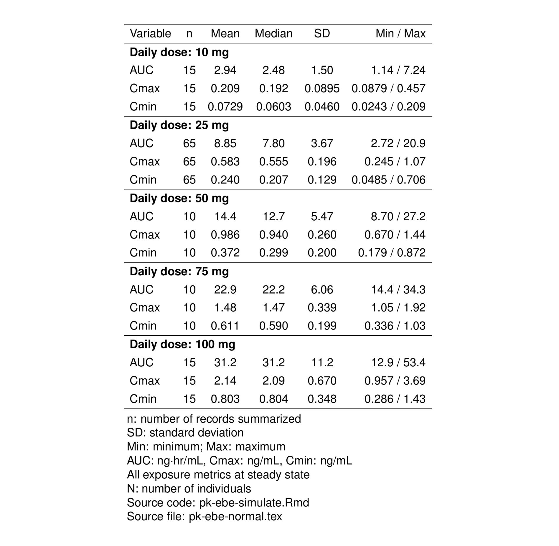
Save the table to the deliv/tables directory
- Recall we set
outputin thest_files()call to set the output file name (a.texfile) - Recall we set the
pmtables.diroption to direct the output to that directory
stable_save(tab) 10 Exposure comparison - renal function groups
In this section, we’ll create a table summarizing exposures by dose level and renal function group.
First, we’ll make the data long with respect to the exposure metrics
pk_long <- pivot_longer(pk, cols = c(Cmax, Cmin, AUC))

head(pk_long)
# A tibble: 6 × 7
STUDY USUBJID ID DOSE RF name value
<chr> <chr> <dbl> <int> <chr> <chr> <dbl>
1 101-DEMO-001 101-DEMO-0010001 1 5 norm Cmax 0.141
2 101-DEMO-001 101-DEMO-0010001 1 5 norm Cmin 0.0457
3 101-DEMO-001 101-DEMO-0010001 1 5 norm AUC 1.90
4 101-DEMO-001 101-DEMO-0010002 2 5 norm Cmax 0.186
5 101-DEMO-001 101-DEMO-0010002 2 5 norm Cmin 0.0707
6 101-DEMO-001 101-DEMO-0010002 2 5 norm AUC 2.66 Now, group by dose level and renal function group and summarize
pk_sum <-
  pk_long %>%
  group_by(DOSE, RF, Metric = name) %>%
  summarise(
    N = n(),
    Median = median(value),
    Min = min(value),
    Max = max(value),
    .groups = "drop"
  )
Subset the PK summary to the doses of interest
compare <- filter(pk_sum, DOSE >= 25 & DOSE <= 75)We use the sig() function from the pmtables package to limit significant digits and render the summary as character data type
compare <- mutate(compare, across(c(Median, Min, Max), sig))Continue to get the data frame ready to generate a table.
We can convert the RF column into a factor with labels coming from the yspec object
compare <- ys_add_factors(compare, spec, RF, .suffix = "f")
count(compare, RF, RFf)
# A tibble: 4 × 3
RF RFf n
<chr> <fct> <int>
1 mild mild 3
2 mod moderate 3
3 norm normal 9
4 sev severe 3compare <- select(compare, DOSE, Metric, Renal = RFf, everything())
compare <- arrange(compare, DOSE, Metric, Renal)
compare <- mutate(compare, DOSEf = paste0(DOSE, " mg daily")) Using the compare data frame, start styling the table
tab2 <-
  compare %>%
  select(-RF, -DOSE) %>%
  st_new() %>%
  st_right(.l = "Metric, Renal") %>%
  st_clear_reps(Metric) %>%
  st_panel("DOSEf", prefix = "Dose:") %>%
  st_notes("AUC: ng$\\cdot$hr/mL, Cmax: ng/mL, Cmin: ng/mL") %>%
  st_notes("All exposure metrics at steady state") %>%
  st_notes("N: number of individuals") %>%
  st_files(
    r = "pk-ebe-simulate.R",
    output = "pk-ebe-compare.tex"
  ) %>% stable()
In the above pipeline
st_rightjustifies columns to the right and customizesMetricandRenalst_clear_repsremoves replicate values in theMetriccolumnst_panelcreates groups of rows into panels with grouping titlest_notesadds table footnotesst_filesattaches source code and output file names
To preview the TeX table as a png graphic, we’ll use st_as_image() from the pmtables package
st_as_image(tab2)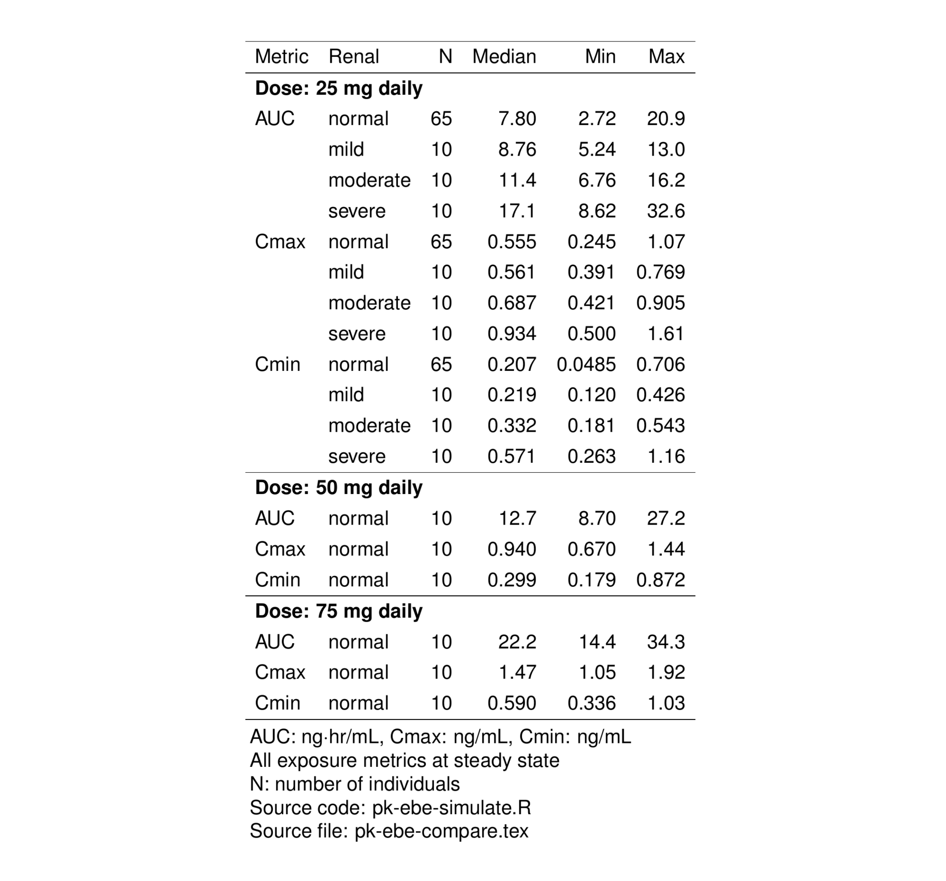
As above, we save the table object which already has the output file name embedded
stable_save(tab2) 11 Preview tables in report environment
On this page, we generated two tables using the pmtables package. Previews of those tables were shown in Figure 1 and Figure 2.
We might also be interested in seeing how the tables appear in our LaTex report template. This can be done with the st2report() function from the pmtables package. The code below won’t render in this website, but you can try it on the tables you create with pmtables.
if(FALSE) {
  st2report(list(tab, tab2), ntex = 2)
}