library(bbr)
library(dplyr)
library(here)

MODEL_DIR <- here("model", "pk")
FIGURE_DIR <- here("deliv", "figure")1 Introduction
Managing the model development process in a traceable and reproducible manner can be a significant challenge. At MetrumRG, we use bbr to streamline this process. bbr is an R package developed by MetrumRG that serves three primary purposes:
- Submit NONMEM® models, particularly for execution in parallel and/or on a high-performance compute (HPC) cluster (e.g. Metworx).
- Parse NONMEM® outputs into R objects to facilitate model evaluation and diagnostics in R.
- Annotate the model development process for easier and more reliable traceability and reproducibility.
This page demonstrates the following bbr functionality:
- Create and submit a model
- Simple model evaluation and diagnostics
- Iterative model development
- Annotation of models with tags, notes, etc.
2 Tools used
2.1 MetrumRG packages
bbr Manage, track, and report modeling activities, through simple R objects, with a user-friendly interface between R and NONMEM®.
2.2 CRAN packages
dplyr A grammar of data manipulation.
3 Outline
This page details a range of tasks typically performed throughout the modeling process such as defining, submitting and annotating models. Typically, our scientists run this code in a scratch pad style script, because it isn’t necessary for the entire coding history for each model to persist. Here, the code used each step of the process is provided as a reference, and a runnable version of this page is available in our Github repository: model-management-demo.Rmd.
If you’re a new bbr user, we recommend you read through the Getting Started vignette before trying to run any code. This vignette includes some setup and configuration (e.g., making sure bbr can find your NONMEM® installation) that needs to be done.
Please note that, for the most part, bbr doesn’t edit the model structure in your control stream. This page walks through a sequence of models that might evolve during a simple modeling project. All modifications to the control streams were made directly by the user in the control stream, and below we include comments asking you to edit your control streams manually.
After working through this content, we recommend reading the Model Run Logs page. The purpose of the Model Run Logs is to provide a high-level overview of the current status of the project, and we show how to leverage the model annotation to summarize your modeling work. Specifically, how to create model run logs using bbr::run_log() to summarize key features of each model (including the descriptions, notes and tag fields), and to provide suggestions for model notes that capture key decision points in the modeling process.
4 Set up
Load required packages and set file paths to your model and figure directories.
5 Model creation and submission
5.1 Control stream
Before using bbr, you’ll need to have a control stream describing your first model. We began this analysis with a simple one compartment model and named our first control stream 100.ctl:
cat(readLines(file.path(MODEL_DIR, "100.ctl")), sep = "\n")$PROB RUN# 100 - fit of Phase I data base model
$INPUT C NUM ID TIME SEQ CMT EVID AMT DV AGE WT HT EGFR ALB BMI SEX AAG
SCR AST ALT CP TAFD TAD LDOS MDV BLQ PHASE
$DATA ../../../data/derived/pk.csv IGNORE=@ IGNORE=(BLQ.EQ.1)
$SUBROUTINE ADVAN2 TRANS2
$PK
;log transformed PK parms
KA = EXP(THETA(1)+ETA(1))
V = EXP(THETA(2)+ETA(2))
CL = EXP(THETA(3)+ETA(3))
S2 = V/1000 ; dose in mcg, conc in mcg/mL
$ERROR
IPRED = F
Y=IPRED*(1+EPS(1))
$THETA ; log values
(-0.69) ; 1 KA (1/hr) - 1.5
(3.5) ; 2 V2 (L) - 60
(1) ; 3 CL (L/hr) - 3.5
$OMEGA BLOCK(3)
0.2 ;ETA(KA)
0.01 0.2 ;ETA(V)
0.01 0.01 0.2 ;ETA(CL)
$SIGMA
0.05 ; 1 pro error
$EST MAXEVAL=9999 METHOD=1 INTER SIGL=9 NSIG=3 PRINT=1 RANMETHOD=P MSFO=./100.MSF
$COV PRINT=E RANMETHOD=P
$TABLE NUM IPRED NPDE CWRES NOPRINT ONEHEADER RANMETHOD=P FILE=100.tab
$TABLE NUM CL V KA ETAS(1:LAST) NOAPPEND NOPRINT ONEHEADER FILE=100par.tab5.2 Create a model object
After creating your control stream, you create a model object. This model object is passed to all of the other bbr functions that submit, summarize, or manipulate models. You can read more about the model object, and the function that creates it, bbr::new_model(), in the Create model object section of the “Getting Started” vignette.
Create your first model:
mod100 <- new_model(file.path(MODEL_DIR, 100))The first argument to new_model() is the path to your model control stream without the file extension. The call above assumes you have a control stream named 100.ctl (or 100.mod) in the MODEL_DIR directory.
5.2.1 The model YAML file
Prior to creating your model object with new_model(), your model directory had two files: the model control stream and the bbi.yaml configuration file (discussed below).
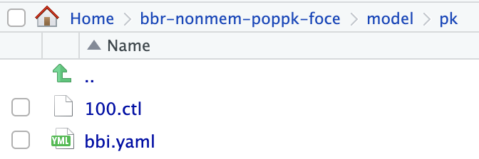
The new_model() function creates a 100.yaml file in your model directory that automatically persists any tags, notes, and other model metadata.
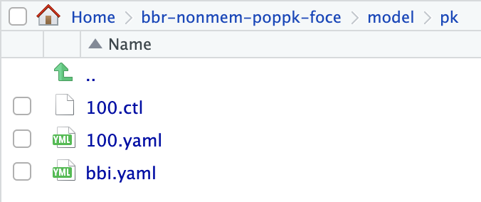
While it’s useful to know that this YAML file exists, you shouldn’t need to interact with it directly (e.g., in the RStudio file tabs). Instead, bbr has a variety of functions (i.e., add_tags() and add_notes(), shown below) that work with the model object to edit the information in the YAML file from your R console.
5.2.2 The bbi.yaml file
Global settings used by bbr are stored in bbi.yaml (located in your model directory). You can read more about this file in the bbi.yaml configuration file section of the “Getting Started” vignette.
5.3 Submitting a model
Now that you have your model object, you can submit it to run with bbr::submit_model().
submit_model(mod100)There are numerous customizations available for submitting models. You can find more detailed information in the bbr documentation and R help:?submit_model and ?modify_bbi_args.
5.3.1 Monitoring submitted models
For models submitted to the SGE grid (the default), you can use system("qstat") to check on your model jobs. In addition, bbr provides some helper functions that show the head and tail (by default, the first 3 and last 5 lines) of specified files and prints them to the console. For example, tail_lst shows the latest status of the lst file and, in this case, indicates the model has finished running.
tail_lst(mod100). Wed 31 Jul 2024 03:33:39 PM EDT
. $PROB RUN# 100 - fit of Phase I data base model
. $INPUT C NUM ID TIME SEQ CMT EVID AMT DV AGE WT HT EGFR ALB BMI SEX AAG
. ...
.
. Elapsed finaloutput time in seconds: 1.38
. #CPUT: Total CPU Time in Seconds, 46.394
. Stop Time:
. Wed 31 Jul 2024 03:38:01 PM EDT6 Summarize model outputs
Once your model has run, you can start looking at the model outputs and creating diagnostics. The bbr::model_summary() function returns an object that contains information parsed from a number of files in the output folder.
sum100 <- model_summary(mod100)
names(sum100)
. [1] "absolute_model_path" "run_details" "run_heuristics"
. [4] "parameters_data" "parameter_names" "ofv"
. [7] "condition_number" "shrinkage_details" "success"This summary object is essentially just a named list that you can explore (e.g., with View(sum100)) and includes everything from the .lst file and a few others.
sum100$run_details$output_files_used. [1] "100.lst" "100.cpu" "100.ext" "100.grd" "100.shk"6.1 High-level model summary
Printing this summary object sum100 to the console shows a high-level summary of the model performance. Further, if you’re using an Rmarkdown, you can print a well formatted version of this summary using the chunk option results = 'asis':
sum100Dataset: ../../../data/derived/pk.csv
Records: 4292 Observations: 3142 Subjects: 160
Objective Function Value (final est. method): 33502.965
Estimation Method(s):
– First Order Conditional Estimation with Interaction
Simulation: No
Heuristic Problem(s) Detected:
– parameter_near_boundary
– hessian_reset
– has_final_zero_gradient
| parameter_names | estimate | stderr | shrinkage |
|---|---|---|---|
| THETA1 | 1.40 | ||
| THETA2 | 4.56 | ||
| THETA3 | 1.04 | ||
| OMEGA(1,1) | 0.0574 | 3.15 | |
| OMEGA(2,2) | 0.0855 | 4.28 | |
| OMEGA(3,3) | 0.173 | 1.15 | |
| SIGMA(1,1) | 0.0882 | 4.09 |
6.2 Simple parameter table
You can also explore this summary object with one of bbr’s helper functions. For example, you can quickly construct a basic parameter table:
sum100 %>% param_estimates(). # A tibble: 10 × 8
. parameter_names estimate stderr random_effect_sd random_effect_sdse fixed
. <chr> <dbl> <dbl> <dbl> <dbl> <lgl>
. 1 THETA1 1.40 NA NA NA FALSE
. 2 THETA2 4.56 NA NA NA FALSE
. 3 THETA3 1.04 NA NA NA FALSE
. 4 OMEGA(1,1) 0.0574 NA 0.240 NA FALSE
. 5 OMEGA(2,1) -0.000183 NA -0.00262 NA FALSE
. 6 OMEGA(2,2) 0.0855 NA 0.292 NA FALSE
. 7 OMEGA(3,1) 0.0704 NA 0.706 NA FALSE
. 8 OMEGA(3,2) 0.0858 NA 0.706 NA FALSE
. 9 OMEGA(3,3) 0.173 NA 0.416 NA FALSE
. 10 SIGMA(1,1) 0.0882 NA 0.297 NA FALSE
. # ℹ 2 more variables: diag <lgl>, shrinkage <dbl>6.3 Investigating heuristics
The summary object printed above showed several of the heuristic problems were flagged when reading the output files. These are not errors per se, but points to check because they could indicate an issue with the model.
The documentation for ?model_summary describes each of these heuristics. There are helper functions like bbr::nm_grd() that pull the gradient file into a tibble. Alternatively, information like the condition number can be extracted from the summary object itself using sum100$condition_number.
The PRDERR flag in the heuristics section means there was a PRDERR file generated by NONMEM® for this run. You can use file.path(get_output_dir(sum100), "PRDERR") to easily get the path to that file, and take a look at it with file.edit() or readLines() to see what the error was.
6.4 Diagnostic plots
During model development, goodness-of-fit (GOF) diagnostic plots are typically generated to assess model fit. We demonstrate how to make these on the Model Diagnostics and Parameterized Reports for Model Diagnostics pages. Our parameterized reports generate a browsable html file including the model summary and all GOF diagnostic plots (in your model directory). They also save out each plot to .pdf files in deliv/figure/{run}/. You can include any plots of particular interest here, for example, this CWRES plot:
knitr::include_graphics(file.path(FIGURE_DIR, "100/100-cwres-combined.pdf"))7 Annotating your model
bbr has some great features that allow you to easily annotate your models. This helps you document your modeling process as you go, and can be easily retrieved later for creating “run logs” that describe the entire analysis (shown later).
A well-annotated model development process does several important things:
- Makes it easy to update collaborators on the state of the project.
- Supports reproducibility and traceability of your results.
- Keeps the project organized, in case you need to return to it at a later date.
The bbr model object contains three annotation fields. The description is a character scalar (i.e., a single string), while notes and tags can contain character vectors of any length. These fields can be used for any purpose but we recommended some patterns below that work for us. These three fields can also be added to the model object at any time (before or after submitting the model).
7.1 Using description
The description field is typically only used for particularly notable models and defaults to NULL if no description is provided. One benefit of this approach is that you can easily filter your Run log to the notable models using dplyr::filter(!is.null(description)).
Descriptions are typically brief, for example, “Base model” or “First covariate model”. We demonstrate the add_description() function for mod102 below.
7.2 Using notes
Notes are often used for free text observations about a particular model. Some modelers leverage notes as “official” annotations that might get pulled into a run log for a final report of some kind, while other modelers prefer to keep them informal and use them primarily for their own reference.
In this example, based on the CWRES plot above, you might add a note like this to your model, and then move on to testing a two-compartment model (model 101, in the next section).
mod100 <- mod100 %>%
add_notes("systematic bias, explore alternate compartmental structure")8 Iterative model development
After running your first model, you can create a new model based on the previous model, using the bbr::copy_model_from() function. This will accomplish several objectives:
- Copy the control stream associated with
.parent_modand rename it according to.new_model. - Create a new model object associated with this new control stream.
- Fill the
based_onfield in the new model object (see the Using based_on vignette). - Optionally, inherit any tags from the parent model.
8.1 Using copy_model_from()
Learn more about this function from ?copy_model_from or the Iteration section of the “Getting Started” vignette.
mod101 <- copy_model_from(
    .parent_mod = mod100,
    .new_model = 101,
    .inherit_tags = TRUE
  )
Though .new_model = 101 is explicitly passed here, this argument can be omitted if you’re naming your models numerically, as in this example. If .new_model is not passed, bbr defaults to incrementing the new model name to the next available integer in the same directory as .parent_mod.
8.1.1 Edit your control stream
As mentioned above, you need to manually edit the new control stream with any modifications. In this case, we updated the model structure from one- to two-compartments.
If you’re using Rstudio, you can easily open your control stream for editing with the following:
mod101 %>%
  get_model_path() %>%
  file.edit()
bbr also has several helper functions to help update your control stream, for example, the defined suffixes can be updated directly from your R console. The update_model_id function updates the defined suffixes from {parent_mod}.{suffix} to {current_mod}.{suffix} in your new control stream for the following file extensions:
- * .MSF
- * .EXT
- * .CHN
- * .tab
- * par.tab
mod101 <- update_model_id(mod101)You can easily look at the differences between control streams of a model and it’s parent model:
model_diff(mod101)@@ 1,10 @@@@ 1,9 @@<$PROBLEM From bbr: see 101.yaml for details>$PROB RUN# 100 - fit of Phase I data base model<~$INPUT C NUM ID TIME SEQ CMT EVID AMT DV AGE WT HT EGFR ALB BMI SEX AAG$INPUT C NUM ID TIME SEQ CMT EVID AMT DV AGE WT HT EGFR ALB BMI SEX AAGSCR AST ALT CP TAFD TAD LDOS MDV BLQ PHASESCR AST ALT CP TAFD TAD LDOS MDV BLQ PHASE<$DATA ../../../data/derived/pk.csv IGNORE=(C='C', BLQ=1)>$DATA ../../../data/derived/pk.csv IGNORE=@ IGNORE=(BLQ.EQ.1)<$SUBROUTINE ADVAN4 TRANS4>$SUBROUTINE ADVAN2 TRANS2$PK$PK@@ 13,34 @@@@ 12,30 @@KA = EXP(THETA(1)+ETA(1))KA = EXP(THETA(1)+ETA(1))<V2 = EXP(THETA(2)+ETA(2))>V = EXP(THETA(2)+ETA(2))CL = EXP(THETA(3)+ETA(3))CL = EXP(THETA(3)+ETA(3))<V3 = EXP(THETA(4))~<Q = EXP(THETA(5))~<S2 = V2/1000 ; dose in mcg, conc in mcg/mL>S2 = V/1000 ; dose in mcg, conc in mcg/mL$ERROR$ERRORIPRED = FIPRED = F~>Y=IPRED*(1+EPS(1))Y=IPRED*(1+EPS(1))$THETA ; log values$THETA ; log values<(0.5) ; 1 KA (1/hr) - 1.5>(-0.69) ; 1 KA (1/hr) - 1.5(3.5) ; 2 V2 (L) - 60(3.5) ; 2 V2 (L) - 60(1) ; 3 CL (L/hr) - 3.5(1) ; 3 CL (L/hr) - 3.5<(4) ; 4 V3 (L) - 70~<(2) ; 5 Q (L/hr) - 4~$OMEGA BLOCK(3)$OMEGA BLOCK(3)0.2 ;ETA(KA)0.2 ;ETA(KA)<0.01 0.2 ;ETA(V2)>0.01 0.2 ;ETA(V)0.01 0.01 0.2 ;ETA(CL)0.01 0.01 0.2 ;ETA(CL)<~$SIGMA$SIGMA0.05 ; 1 pro error0.05 ; 1 pro error<$EST MAXEVAL=9999 METHOD=1 INTER SIGL=6 NSIG=3 PRINT=1 RANMETHOD=P MSFO=./101.MSF>$EST MAXEVAL=9999 METHOD=1 INTER SIGL=9 NSIG=3 PRINT=1 RANMETHOD=P MSFO=./100.MSF$COV PRINT=E RANMETHOD=P$COV PRINT=E RANMETHOD=P<$TABLE NUM IPRED NPDE CWRES NOPRINT ONEHEADER RANMETHOD=P FILE=101.tab>$TABLE NUM IPRED NPDE CWRES NOPRINT ONEHEADER RANMETHOD=P FILE=100.tab<$TABLE NUM CL V2 Q V3 KA ETAS(1:LAST) NOAPPEND NOPRINT ONEHEADER FILE=101par.tab>$TABLE NUM CL V KA ETAS(1:LAST) NOAPPEND NOPRINT ONEHEADER FILE=100par.tab
8.1.3 Add notes
In this example, after running model 101 and looking at the model outputs and diagnostics (as described above for model 100), we can see there is a correlation between eta-V2 and weight. This is the type of feature we might add as a note to our model object before moving on to the next model.
knitr::include_graphics(file.path(FIGURE_DIR, "101/101-eta-all-cont-cov.pdf"))mod101 <- mod101 %>%
add_notes("eta-V2 shows correlation with weight, consider adding allometric weight")8.2 Adding weight covariate effects
Next we create a new model, based on 101, and add some covariate effects. In this example, we demonstrate how you can use add_tags() instead of replace_tag() to add new tags rather than replace any existing tag. See tags for details on the different functions for interacting with tags.
Create a new model by copying model 101, inherit tags from the parent model and add new tags describing the covariate effects:
mod102 <- copy_model_from(
    mod101,
    .new_model = 102,
    .inherit_tags = TRUE
  ) %>%
  add_tags(c(
    TAGS$cov_cl_wt_fixed,
    TAGS$cov_v2_wt_fixed,
    TAGS$cov_q_wt_fixed,
    TAGS$cov_v3_wt_fixed
  ))
Check the differences between mod102 and it’s parent (mod101):
model_diff(mod102)@@ 1,3 @@@@ 1,3 @@<$PROBLEM From bbr: see 102.yaml for details>$PROBLEM From bbr: see 101.yaml for details$INPUT C NUM ID TIME SEQ CMT EVID AMT DV AGE WT HT EGFR ALB BMI SEX AAG$INPUT C NUM ID TIME SEQ CMT EVID AMT DV AGE WT HT EGFR ALB BMI SEX AAG@@ 12,14 @@@@ 12,9 @@;log transformed PK parms;log transformed PK parms<V2WT = LOG(WT/70)~<CLWT = LOG(WT/70)*0.75~<V3WT = LOG(WT/70)~<QWT = LOG(WT/70)*0.75~<~KA = EXP(THETA(1)+ETA(1))KA = EXP(THETA(1)+ETA(1))<V2 = EXP(THETA(2)+V2WT+ETA(2))>V2 = EXP(THETA(2)+ETA(2))<CL = EXP(THETA(3)+CLWT+ETA(3))>CL = EXP(THETA(3)+ETA(3))<V3 = EXP(THETA(4)+V3WT)>V3 = EXP(THETA(4))<Q = EXP(THETA(5)+QWT)>Q = EXP(THETA(5))S2 = V2/1000 ; dose in mcg, conc in mcg/mLS2 = V2/1000 ; dose in mcg, conc in mcg/mL@@ 42,9 @@@@ 37,10 @@0.01 0.01 0.2 ;ETA(CL)0.01 0.01 0.2 ;ETA(CL)~>$SIGMA$SIGMA0.05 ; 1 pro error0.05 ; 1 pro error<$EST MAXEVAL=9999 METHOD=1 INTER SIGL=6 NSIG=3 PRINT=1 RANMETHOD=P MSFO=./102.MSF>$EST MAXEVAL=9999 METHOD=1 INTER SIGL=6 NSIG=3 PRINT=1 RANMETHOD=P MSFO=./101.MSF$COV PRINT=E RANMETHOD=P$COV PRINT=E RANMETHOD=P<$TABLE NUM IPRED NPDE CWRES NOPRINT ONEHEADER RANMETHOD=P FILE=102.tab>$TABLE NUM IPRED NPDE CWRES NOPRINT ONEHEADER RANMETHOD=P FILE=101.tab<$TABLE NUM CL V2 Q V3 KA ETAS(1:LAST) NOAPPEND NOPRINT ONEHEADER FILE=102par.tab>$TABLE NUM CL V2 Q V3 KA ETAS(1:LAST) NOAPPEND NOPRINT ONEHEADER FILE=101par.tab
Submit the model:
submit_model(mod102)And, after looking at the model diagnostics (as shown above), add a note to this model:
mod102 <- mod102 %>%
  add_notes("Allometric scaling with weight reduced eta-V2 correlation with weight. Will consider additional RUV structures")
9 Comparing error structures
During model development you may reach a “fork in the road” and want to test two different options forward. Here we demonstrate this with two different potential error structures: additive error only (mod103), or combined proportional and additive error terms (mod104). Both new models use mod102 as the .parent_mod argument in copy_model_from().
mod103 <- copy_model_from(
    mod102,
    .new_model = 103,
    .inherit_tags = TRUE
  ) %>%
  replace_tag(TAGS$proportional_ruv, TAGS$additive_ruv)

mod104 <- copy_model_from(
    mod102,
    .new_model = 104,
    .inherit_tags = TRUE
  ) %>%
  replace_tag(TAGS$proportional_ruv, TAGS$combined_ruv)
Remember the control streams are updated manually and then you can see the changes made to the additive error model (you also update some parameter estimates, mod103):
model_diff(mod103)@@ 1,3 @@@@ 1,3 @@<$PROBLEM From bbr: see 103.yaml for details>$PROBLEM From bbr: see 102.yaml for details$INPUT C NUM ID TIME SEQ CMT EVID AMT DV AGE WT HT EGFR ALB BMI SEX AAG$INPUT C NUM ID TIME SEQ CMT EVID AMT DV AGE WT HT EGFR ALB BMI SEX AAG@@ 27,24 @@@@ 27,24 @@$ERROR$ERRORIPRED = FIPRED = F<Y=IPRED+EPS(1)>Y=IPRED*(1+EPS(1))$THETA ; log values$THETA ; log values<(0.42) ; 1 KA (1/hr) - 1.5>(0.5) ; 1 KA (1/hr) - 1.5<(4.06) ; 2 V2 (L) - 60>(3.5) ; 2 V2 (L) - 60<(1.11) ; 3 CL (L/hr) - 3.5>(1) ; 3 CL (L/hr) - 3.5<(4.28) ; 4 V3 (L) - 70>(4) ; 4 V3 (L) - 70<(1.31) ; 5 Q (L/hr) - 4>(2) ; 5 Q (L/hr) - 4$OMEGA BLOCK(3)$OMEGA BLOCK(3)<0.02 ;ETA(KA)>0.2 ;ETA(KA)<0.01 0.02 ;ETA(V2)>0.01 0.2 ;ETA(V2)<0.01 0.01 0.09 ;ETA(CL)>0.01 0.01 0.2 ;ETA(CL)$SIGMA$SIGMA<1000 ; 1 add error>0.05 ; 1 pro error<$EST MAXEVAL=9999 METHOD=1 INTER SIGL=6 NSIG=3 PRINT=1 RANMETHOD=P MSFO=./103.MSF>$EST MAXEVAL=9999 METHOD=1 INTER SIGL=6 NSIG=3 PRINT=1 RANMETHOD=P MSFO=./102.MSF$COV PRINT=E RANMETHOD=P$COV PRINT=E RANMETHOD=P<$TABLE NUM IPRED NPDE CWRES NOPRINT ONEHEADER RANMETHOD=P FILE=103.tab>$TABLE NUM IPRED NPDE CWRES NOPRINT ONEHEADER RANMETHOD=P FILE=102.tab<$TABLE NUM CL V2 Q V3 KA ETAS(1:LAST) NOAPPEND NOPRINT ONEHEADER FILE=103par.tab>$TABLE NUM CL V2 Q V3 KA ETAS(1:LAST) NOAPPEND NOPRINT ONEHEADER FILE=102par.tab
As with model 103, model 104 is also based on 102 but it incorporates changes for a combined error model (mod104).
model_diff(mod104)@@ 1,3 @@@@ 1,3 @@<$PROBLEM From bbr: see 104.yaml for details>$PROBLEM From bbr: see 102.yaml for details$INPUT C NUM ID TIME SEQ CMT EVID AMT DV AGE WT HT EGFR ALB BMI SEX AAG$INPUT C NUM ID TIME SEQ CMT EVID AMT DV AGE WT HT EGFR ALB BMI SEX AAG@@ 27,5 @@@@ 27,5 @@$ERROR$ERRORIPRED = FIPRED = F<Y=IPRED*(1+EPS(1))+EPS(2)>Y=IPRED*(1+EPS(1))$THETA ; log values$THETA ; log values@@ 44,8 @@@@ 44,7 @@$SIGMA$SIGMA0.05 ; 1 pro error0.05 ; 1 pro error<0.05 ; 2 add error~<$EST MAXEVAL=9999 METHOD=1 INTER SIGL=6 NSIG=3 PRINT=1 RANMETHOD=P MSFO=./104.MSF>$EST MAXEVAL=9999 METHOD=1 INTER SIGL=6 NSIG=3 PRINT=1 RANMETHOD=P MSFO=./102.MSF$COV PRINT=E RANMETHOD=P$COV PRINT=E RANMETHOD=P<$TABLE NUM IPRED NPDE CWRES NOPRINT ONEHEADER RANMETHOD=P FILE=104.tab>$TABLE NUM IPRED NPDE CWRES NOPRINT ONEHEADER RANMETHOD=P FILE=102.tab<$TABLE NUM CL V2 Q V3 KA ETAS(1:LAST) NOAPPEND NOPRINT ONEHEADER FILE=104par.tab>$TABLE NUM CL V2 Q V3 KA ETAS(1:LAST) NOAPPEND NOPRINT ONEHEADER FILE=102par.tab
9.1 Submit models in batches
In addition to submit_model(), which takes a single model object, bbr also has a submit_models() function, which takes a list of model objects. This is especially useful for tasks like running a bootstrap, or for re-running a batch of models, as shown at the bottom of this page. However, it can also be used to submit two models at once:
submit_models(list(mod103, mod104))9.2 Compare objective functions with summary_log()
The bbr::summary_log() function essentially runs bbr::model_summary() (shown in the “Summarize model outputs” section above) on all models in the specified directory, and parses the outputs into a tibble. This is very useful for comparing multiple models at any point in the project.
The ?summary_log help page provides details on what is parsed into this bbi_summary_log_df tibble, and the Creating summary log vignette gives additional tips on how to effectively use this function. For example, the .include argument filters to only models which match the run names passed to .include. (You can also pass a vector of tags to .include to filter to only models with those tags.) This, and other related functionality, is also discussed in more detail on the
summary_log(MODEL_DIR, .include = 102:104) %>%
  select(
    run,
    ofv,
    param_count,
    condition_number,
    any_heuristics
) %>% knitr::kable()| run | ofv | param_count | condition_number | any_heuristics |
|---|---|---|---|---|
| 102 | 30997.91 | 12 | 29.8235 | FALSE |
| 103 | 36411.27 | 12 | 88.6217 | FALSE |
| 104 | 30997.71 | 13 | 30.0777 | FALSE |
Based on these metrics, you can begin making decisions about the error structures tested, and you can make notes about these decisions:
mod103 <- mod103 %>%
  add_notes("Additive only RUV performs poorly and will not be considered going forward.")

mod104 <- mod104 %>%
  add_notes("Combined RUV performs only slightly better than proportional only, should look at parameter estimates for 104")
9.3 Looking at OMEGA and SIGMA
bbr provides helpers for extracting the OMEGA and SIGMA matrices. You can pass the bbi_nonmem_summary object, returned from model_summary(), to one of the get_*() helpers.
sum104 <- model_summary(mod104)
get_omega(sum104)
. OMEGA_1 OMEGA_2 OMEGA_3
. OMEGA_1 0.2201550 0.0688803 0.1338700
. OMEGA_2 0.0688803 0.0827208 0.0735232
. OMEGA_3 0.1338700 0.0735232 0.1693070get_sigma(sum104). SIGMA_1 SIGMA_2
. SIGMA_1 0.0397749 0.000000
. SIGMA_2 0.0000000 0.841006You can also filter the output of param_estimates() to see a bit more detail about the SIGMA parameters estimated in model 104.
sum104 %>%
  param_estimates() %>%
filter(grepl("SIGMA", parameter_names) & !fixed) %>% knitr::kable()| parameter_names | estimate | stderr | random_effect_sd | random_effect_sdse | fixed | diag | shrinkage |
|---|---|---|---|---|---|---|---|
| SIGMA(1,1) | 0.0397749 | 0.0012579 | 0.199436 | 0.0031536 | FALSE | TRUE | 5.28286 |
| SIGMA(2,2) | 0.8410060 | 2.8770600 | 0.917064 | 1.5686200 | FALSE | TRUE | 5.28286 |
Based on these parameter estimates, you might decide not to proceed with the combined error model because the additive error parameter contains zero. You can make a note of this, and add a description to mod102 to denote that it’s your base model.
mod104 <- mod104 %>%
    add_notes("CI for additive error parameter contains zero and will not be used going forward")

mod102 <- mod102 %>%
  add_notes("Proportional RUV performed best over additive (103) and combined (104)") %>%
  add_description("Base Model")
10 Final models
10.1 Including covariate effects
After identifying our base model, we tested some pre-specified covariates:
mod105 <- copy_model_from(
    mod102,
    .new_model = 105,
    .inherit_tags = TRUE
  )
Remember to edit the control stream manually:
model_diff(mod105)@@ 1,3 @@@@ 1,3 @@<$PROBLEM From bbr: see 105.yaml for details>$PROBLEM From bbr: see 102.yaml for details$INPUT C NUM ID TIME SEQ CMT EVID AMT DV AGE WT HT EGFR ALB BMI SEX AAG$INPUT C NUM ID TIME SEQ CMT EVID AMT DV AGE WT HT EGFR ALB BMI SEX AAG@@ 14,6 @@@@ 14,4 @@V2WT = LOG(WT/70)V2WT = LOG(WT/70)CLWT = LOG(WT/70)*0.75CLWT = LOG(WT/70)*0.75<CLEGFR = LOG(EGFR/90)*THETA(6)~<CLAGE = LOG(AGE/35)*THETA(7)~V3WT = LOG(WT/70)V3WT = LOG(WT/70)QWT = LOG(WT/70)*0.75QWT = LOG(WT/70)*0.75@@ 21,5 @@@@ 19,5 @@KA = EXP(THETA(1)+ETA(1))KA = EXP(THETA(1)+ETA(1))V2 = EXP(THETA(2)+V2WT+ETA(2))V2 = EXP(THETA(2)+V2WT+ETA(2))<CL = EXP(THETA(3)+CLWT+CLEGFR+CLAGE+ETA(3))>CL = EXP(THETA(3)+CLWT+ETA(3))V3 = EXP(THETA(4)+V3WT)V3 = EXP(THETA(4)+V3WT)Q = EXP(THETA(5)+QWT)Q = EXP(THETA(5)+QWT)@@ 37,7 @@@@ 35,6 @@(4) ; 4 V3 (L) - 70(4) ; 4 V3 (L) - 70(2) ; 5 Q (L/hr) - 4(2) ; 5 Q (L/hr) - 4<(1) ; 6 CL (L/hr)~<(1) ; 7 CL (L/hr)~~>$OMEGA BLOCK(3)$OMEGA BLOCK(3)0.2 ;ETA(KA)0.2 ;ETA(KA)@@ 48,6 @@@@ 45,6 @@0.05 ; 1 pro error0.05 ; 1 pro error<$EST MAXEVAL=9999 METHOD=1 INTER SIGL=6 NSIG=3 PRINT=1 RANMETHOD=P MSFO=./105.MSF>$EST MAXEVAL=9999 METHOD=1 INTER SIGL=6 NSIG=3 PRINT=1 RANMETHOD=P MSFO=./102.MSF$COV PRINT=E RANMETHOD=P$COV PRINT=E RANMETHOD=P<$TABLE NUM IPRED NPDE CWRES NOPRINT ONEHEADER RANMETHOD=P FILE=105.tab>$TABLE NUM IPRED NPDE CWRES NOPRINT ONEHEADER RANMETHOD=P FILE=102.tab<$TABLE NUM CL V2 Q V3 KA ETAS(1:LAST) NOAPPEND NOPRINT ONEHEADER FILE=105par.tab>$TABLE NUM CL V2 Q V3 KA ETAS(1:LAST) NOAPPEND NOPRINT ONEHEADER FILE=102par.tab
10.2 Adding bbi arguments and parallelization
There are a number of bbi arguments available to modify how models are run. These can be set globally in the bbi.yaml file (see bbi.yaml configuration file section of the “Getting Started” vignette) or bbi arguments can be attached to the model object. Assigning the arguments to the model object means they’ll be applied each time the model is submitted. See the section on Passing arguments to bbiin the “Getting Started” vignette for more details, and a list of valid arguments.
These bbi arguments are also how you run your model in parallel (see Running NONMEM in Parallel: bbr Tips and Tricks vignette for more details).
Here we demonstrate adding arguments that are passed to bbi, submitting the model to run, then updating the tags and notes while waiting for the model to run:
mod105 <- mod105 %>% add_bbi_args(list(clean_lvl = 0))

submit_model(mod105)

mod105 <- mod105 %>%
  add_tags(c(
    TAGS$cov_cl_egfr,
    TAGS$cov_cl_age
  )) %>%
  add_notes("Pre-specified covariate model")
10.3 Making final adjustments
Assume you decide on a final model but one of your collaborators is interested in adding the effect albumin to CL. You might copy the covariate model (mod105), add a new tag for the new covariate effect and note the purpose of the model:
mod106 <- copy_model_from(
    mod105,
    .new_model = 106,
    .inherit_tags = TRUE
  ) %>%
  add_tags(TAGS$cov_cl_alb) %>%
  add_notes("Collaborator was interested in adding Albumin to CL")
Edit the control stream manually and submit the model.
submit_model(mod106)Below we show some different ways you can compare these two model outputs to help determine whether 106 is an improvement on 105, and which will be the final model.
10.3.1 Model heuristics
You can use bbr::summary_log() to compare objective functions and check for potential heuristics problems. The ?summary_log help page details which heuristics are checked.
summary_log(MODEL_DIR, .include = 105:106) %>%
select(run, ofv, condition_number, any_heuristics) %>% knitr::kable()| run | ofv | condition_number | any_heuristics |
|---|---|---|---|
| 105 | 30928.82 | 53.8963 | FALSE |
| 106 | 30904.41 | 48.5060 | FALSE |
In this case, you can see no heuristics have been triggered for either model.
10.3.2 Comparing parameter estimates
You might compare the parameter estimates between the two models. You can use bbr::param_estimates() to generate a tibble for each model, and then join them together with some help from dplyr:
params106 <- mod106 %>% model_summary() %>% param_estimates() %>% select(1:3)
params105 <- mod105 %>% model_summary() %>% param_estimates() %>% select(1:3)

full_join(
  params106,
  params105,
  by = "parameter_names",
  suffix = c("_106", "_105")
) %>%
  mutate(across(where(is.numeric), pmtables::sig)) %>%
knitr::kable()| parameter_names | estimate_106 | stderr_106 | estimate_105 | stderr_105 |
|---|---|---|---|---|
| THETA1 | 0.443 | 0.0643 | 0.430 | 0.0624 |
| THETA2 | 4.12 | 0.0275 | 4.12 | 0.0277 |
| THETA3 | 1.17 | 0.0280 | 1.13 | 0.0294 |
| THETA4 | 4.21 | 0.0190 | 4.21 | 0.0191 |
| THETA5 | 1.28 | 0.0348 | 1.29 | 0.0350 |
| THETA6 | 0.485 | 0.0395 | 0.456 | 0.0424 |
| THETA7 | -0.0377 | 0.0635 | 0.000531 | 0.0745 |
| THETA8 | 0.419 | 0.0863 | NA | NA |
| OMEGA(1,1) | 0.219 | 0.0526 | 0.216 | 0.0509 |
| OMEGA(2,1) | 0.0668 | 0.0194 | 0.0679 | 0.0195 |
| OMEGA(2,2) | 0.0824 | 0.00981 | 0.0835 | 0.00997 |
| OMEGA(3,1) | 0.121 | 0.0224 | 0.128 | 0.0222 |
| OMEGA(3,2) | 0.0703 | 0.00918 | 0.0739 | 0.00982 |
| OMEGA(3,3) | 0.114 | 0.0128 | 0.129 | 0.0154 |
| SIGMA(1,1) | 0.0399 | 0.00123 | 0.0399 | 0.00123 |
10.3.3 Review diagnostic plots
As mentioned above, we demonstrate how to make GOF diagnostic plots on the Model Diagnostics and Parameterized Reports for Model Diagnostics pages. Our parameterized reports generate a browsable html file (in your model directory: model/pk/{run}) and save out each GOF plot to .pdf files (in your figure directory: deliv/figure/{run}/).
Assuming you have generate the GOF plots for your two models, you can compare the _eta_pairs.pdf plots between the two models.
Model 105
knitr::include_graphics(file.path(FIGURE_DIR, "105/105-eta-pairs.pdf"))Model 106
knitr::include_graphics(file.path(FIGURE_DIR, "106/106-eta-pairs.pdf"))10.3.4 Choose final model
After checking your model heuristics, parameter estimates, and GOF plots, the final model was determined to be run 106. You can identify this model as the “final model” in the description field so that it can easily be identified as a key model when looking at the run log later.
mod106 <- mod106 %>%
  add_description("Final Model")
10.3.5 Star models of note
You can also add a “star” to notable models. This can be useful later for organizing your models. For example, this is used for filtering to only starred models when looking at the tibble returned run_log() in Model Run Logs. Below, we star the base model and the final model.
mod102 <- add_star(mod102)
mod106 <- add_star(mod106)
11 Submit models to be re-run
There are cases when you may have to re-run some or all of your models. For example, maybe your model or data files changed since the model was last run. You can check this using either the bbr::config_log() function or with bbr functions that track model lineage; examples of both these approaches are shown in the Using based_on vignette.
To re-run a single model, simply pass .overwrite = TRUE to the submit_model() call.
submit_model(mod100, .overwrite=TRUE)To re-run a group of models, pass .overwrite = TRUE to the submit_models() call.
mods <- purrr::map(
  file.path(MODEL_DIR, 100:106),
  read_model
)
submit_models(mods, .overwrite=TRUE)
12 Other resources
The following script from the Github repository is discussed on this page. If you’re interested running this code, visit the About the Github Repo page first.
- Runnable version of the examples on this page:
model-management-demo.Rmd