library(tidyverse)
library(pmparams)
library(pmtables)
library(here)
library(bbr)
library(magrittr)
library(yaml)
library(glue)1 Introduction
Generating clear, well-formatted parameter tables for your NONMEM® model is an important part of reporting your model results, but it is often a tedious, time-consuming process. Here we show how to quickly and simply create parameter tables by leveraging a few intuitive functions designed to:
- Read in your model parameters from various NONMEM® output files
- Describe your model parameters in a YAML file
- Leverage
pmparamsto back-transform any parameters estimated in other domains (e.g., log- or logit-transformed variables), and calculate additional summary statistics (e.g., 95% confidence intervals, coefficient of variation (CV), etc.) - Format the data for a Latex report
MetrumRG reports are written in Latex, so this code focuses on making tables formatted for Latex reports. The tex files can also potentially be displayed in an Rmarkdown file, but they’re not suitable for reports generated in programs like Microsoft Word. However, if you want to use our code to configure a parameter table from the NONMEM® output files for use in other programs, you could save the parameter dataframe out to a csv prior to the step turning it into a tex table.
2 Tools used
2.1 MetrumRG packages
pmparams Extract, organize, transform, and present parameter estimates.
pmtables Create summary tables commonly used in pharmacometrics and turn any R table into a highly customized tex table.
bbr Manage, track, and report modeling activities, through simple R objects, with a user-friendly interface between R and NONMEM®.
2.2 CRAN packages
dplyr A grammar of data manipulation.
3 Outline
This page focuses on making parameter tables for the final model (run 106), including how to create them for a single model run and for the bootstrap runs. Descriptions of the parameters are given in the parameter key YAML file (pk-parameter-key.yaml), and that single YAML can be used in multiple scripts.
4 Set up
4.1 Load required packages
4.2 Other set up
4.3 Model parameter specifications
To run the code on this page, you first need to write a parameter key that tells R how to interpret your parameter values. Our code requires four arguments for each parameter:
abb- abbreviation for model parameter (we use latex coding)desc- parameter description to appearpanel- the table panel the parameter should appear undertrans- definition of how the parameter should be transformed
For example:
THETA1
  abb: "KA (1/h)"
  desc: "First order absorption rate constant"
  panel: struct
  trans: logTrans
We provide some built-in options for the panel and trans arguments, but you can expand these if needed.
We chose to describe all model parameters in a separate pk-parameter-key.yaml YAML file. The advantage is that, depending how your model development progressed, you can potentially use the same parameter key for the base model, final model and bootstrap model parameter tables.
pathKey <- here("script", "pk-parameter-key.yaml")A more detailed walk-through of generating the parameter key is available here: Creating a Parameter Key. Or take a look at pk-parameter-key.yaml which includes some brief instructions at the top.
5 Create final model parameter tables
5.1 Read in model
sum <- read_model(here("model/pk/106")) %>%
        model_summary()
sum %>% param_estimates()
# A tibble: 15 × 8
parameter_names estimate stderr random_effect_sd random_effect_sdse fixed
<chr> <dbl> <dbl> <dbl> <dbl> <lgl>
1 THETA1 0.443 0.0643 NA NA FALSE
2 THETA2 4.12 0.0275 NA NA FALSE
3 THETA3 1.17 0.0280 NA NA FALSE
4 THETA4 4.21 0.0190 NA NA FALSE
5 THETA5 1.28 0.0348 NA NA FALSE
6 THETA6 0.485 0.0395 NA NA FALSE
7 THETA7 -0.0377 0.0635 NA NA FALSE
8 THETA8 0.419 0.0863 NA NA FALSE
9 OMEGA(1,1) 0.219 0.0526 0.468 0.0562 FALSE
10 OMEGA(2,1) 0.0668 0.0194 0.498 0.0998 FALSE
11 OMEGA(2,2) 0.0824 0.00981 0.287 0.0171 FALSE
12 OMEGA(3,1) 0.121 0.0224 0.767 0.0823 FALSE
13 OMEGA(3,2) 0.0703 0.00918 0.725 0.0418 FALSE
14 OMEGA(3,3) 0.114 0.0128 0.338 0.0189 FALSE
15 SIGMA(1,1) 0.0399 0.00123 0.200 0.00309 FALSE
# ℹ 2 more variables: diag <lgl>, shrinkage <dbl>5.2 Format the parameters for the report
To generate a report-ready table we pass the sum object through two pmparams functions
define_param_tablejoins the parameter estimates from the bbr model summary objectsumto parameter key data frame.format_param_tableperforms some house-keeping based on the new parameter key information, calculates any summary statistics (the 95% confidence intervals are calculated by default), and formats the values for the report.
We explain these functions in more detail below, but we tend to run both functions in a single call to format the data:
param_df <- sum  %>%
  define_param_table(.key = pathKey) %>%
  format_param_table()

param_df %>% select(-type)
# A tibble: 15 × 6
abb greek desc value shrinkage ci_95
<chr> <glue> <chr> <glu> <chr> <chr>
1 KA (1/h) $\exp(\theta_{1})$ First order absorption… 1.56 - 1.37…
2 V2/F (L) $\exp(\theta_{2})$ Apparent central volume 61.5 - 58.3…
3 CL/F (L/h) $\exp(\theta_{3})$ Apparent clearance 3.23 - 3.06…
4 V3/F (L) $\exp(\theta_{4})$ Apparent peripheral vo… 67.3 - 64.9…
5 Q/F (L/h) $\exp(\theta_{5})$ Apparent intercompartm… 3.61 - 3.37…
6 CL/F ~ eGFR $\theta_{6}$ eGFR effect on CL/F 0.485 - 0.40…
7 CL/F ~ Age $\theta_{7}$ Age effect on CL/F $-$0… - $-$0…
8 CL/F ~ ALB $\theta_{8}$ Serum albumin effect o… 0.419 - 0.25…
9 IIV-KA $\Omega_{(1,1)}$ Variance of absorption 0.21… 14.4 0.11…
10 IIV-V2/F $\Omega_{(2,2)}$ Variance of central vo… 0.08… 5.50 0.06…
11 IIV-CL/F $\Omega_{(3,3)}$ Variance of clearance 0.11… 1.25 0.08…
12 V2/F-KA $\Omega_{(2,1)}$ Covariance of V2/F - KA 0.06… - 0.02…
13 CL/F-KA $\Omega_{(3,1)}$ Covariance of CL/F - KA 0.12… - 0.07…
14 CL/F-V2/F $\Omega_{(3,2)}$ Covariance of CL/F - V… 0.07… - 0.05…
15 Proportional $\Sigma_{(1,1)}$ Variance 0.03… 5.01 0.03…While we chose to pass define_param_table the bbr model summary sum, you could also pass in the model path or a data frame of parameter estimates. Similarly, we chose to pass define_param_table the path to the parameter key but you could also provide a parameter key data frame.
5.3 Functions used to format the parameters
We use functions in pmparams package to format parameters. Briefly:
define_param_table
- extracts all parameter estimates.
- makes a name column without any punctuation.
- joins parameter details from the parameter key - note this is an inner_join, so only parameters included in the model output and parameter key will be kept in the table. This was done so that, if your base and final model used the same structural THETAs and random parameters, the same parameter key could be used for both. The additional covariate THETAs defined in the parameter key YAML would simply be ignored when creating the base model parameter table. However, if you change any of the THETA/OMEGA/SIGMAs defined in the base model when fitting the final model you will need a second parameter key for the final model.
- checks whether parameters with special transformation rules were defined correctly. For example, for logit transformed variables, the code expects to see the trans (transform) column including the associated THETA value separated with a tilde symbol, e.g., logitOmSD ~ THETA3.
- makes a series of TRUE/FALSE columns that are subsequently used by
format_param_tableto easily distinguish how each row should be handled. - determines a value (or estimate) for each model parameter and it’s associated metric:
- THETA = estimate only
- OMEGA diagonals = variance [%CV]
- OMEGA off-diagonals = covariance [correlation coefficient]
- SIGMA diagonal proportional = variance [%CV]
- SIGMA diagonal additive = variance [SD]
- calculates the upper and lower values of the 95% confidence intervals (CIs). If you want to use a different CI, provide CI and its corresponding z-score (i.e. ci = 85, zscore = 1.440).
format_param_table
- formats the parameters ready for the final table. This potentially includes back transforming parameters and their CIs, rounding parameters using pmtables::sig, and combining columns.
- formats the THETA/OMEGA/SIGMA values to display as greek letters in Latex, with subscript numbers, and where necessary, the transformation applied to that parameter.
- determines which panel of the final table the parameter should be displayed in. This is informed by the panel argument you defined in your parameter key. Note that there are a finite number of options included by default (see below) but you can include additional panels as needed.
- panel==“struct” ~ Structural model parameters
- panel==“cov” ~ Covariate effect parameters
- panel==“IIV” (and a diagonal omega) ~ Interindividual variance parameters
- panel==“IOV” (and a diagonal omega) ~ Interoccasion variance parameters
- Off-diagonal omegas have the panel name ~ Interindividual covariance parameters
- panel == “RV” ~ Residual variance
- selects columns for final tables. Default selects “type”, “abb”, “greek”, “desc”, “value”, “ci”, “shrinkage”. To return all columns, specify “all” for .select_cols
5.4 Create tex versions of the parameter tables
As mentioned above, our reports are written in Latex, so we now convert the param_df to two Latex report-ready tex tables using the pmtables package: one table for fixed effects and one table for random effects.
5.4.1 Fixed effect parameter table
fixed = param_df %>%
  filter(str_detect(type, "Struct") |
           str_detect(type, "effect")) %>%
  select(-shrinkage) %>%
  st_new() %>%
  st_panel("type") %>%
  st_center(desc = col_ragged(5.5),
            abb = "l") %>%
  st_blank("abb", "greek", "desc") %>%
  st_rename("Estimate" = "value",
            "95\\% CI" = "ci_95") %>%
  st_files(output = "pk-param-final-fixed.tex") %>%
  st_notes("Parameters estimated in the log-domain were
           back-transformed for clarity") %>%
  st_notes("Abbreviations: CI = confidence intervals;
                        SE = standard error") %>%
  st_notes("Confidence intervals = estimate $\\pm$ 1.96 $\\cdot$ SE") %>%
  st_noteconf(type = "minipage", width = 1) %>%
  stable() %>%
  stable_save()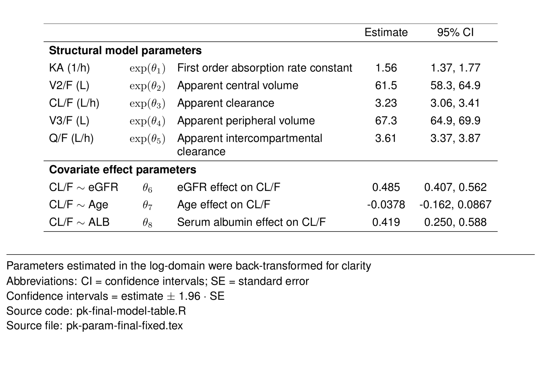
5.4.2 Random effect parameter table
random = param_df %>%
  filter(str_detect(greek, "Omega") |
           str_detect(type, "Resid")) %>%
  select(-desc) %>%
  st_new %>%
  st_panel("type") %>%
  st_center(abb = "l") %>%
  st_blank("abb", "greek") %>%
  st_rename("Estimate" = "value",
            "95\\% CI" = "ci_95",
            "Shrinkage (\\%)" = "shrinkage") %>%
  st_files(output = "pk-param-final-random.tex") %>%
  st_notes("Abbreviations: CI = confidence intervals;
                        Corr = Correlation coefficient;
                        CV = coefficient of variation;
                        SD = standard deviation;
                        SE = standard error") %>%
  st_notes("CV\\% of log-normal omegas = sqrt(exp(estimate) - 1) $\\cdot$ 100") %>%
  st_notes("CV\\% of sigma = sqrt(estimate) $\\cdot$ 100") %>%
  st_noteconf(type = "minipage", width = 1) %>%
  stable() %>%
  stable_save()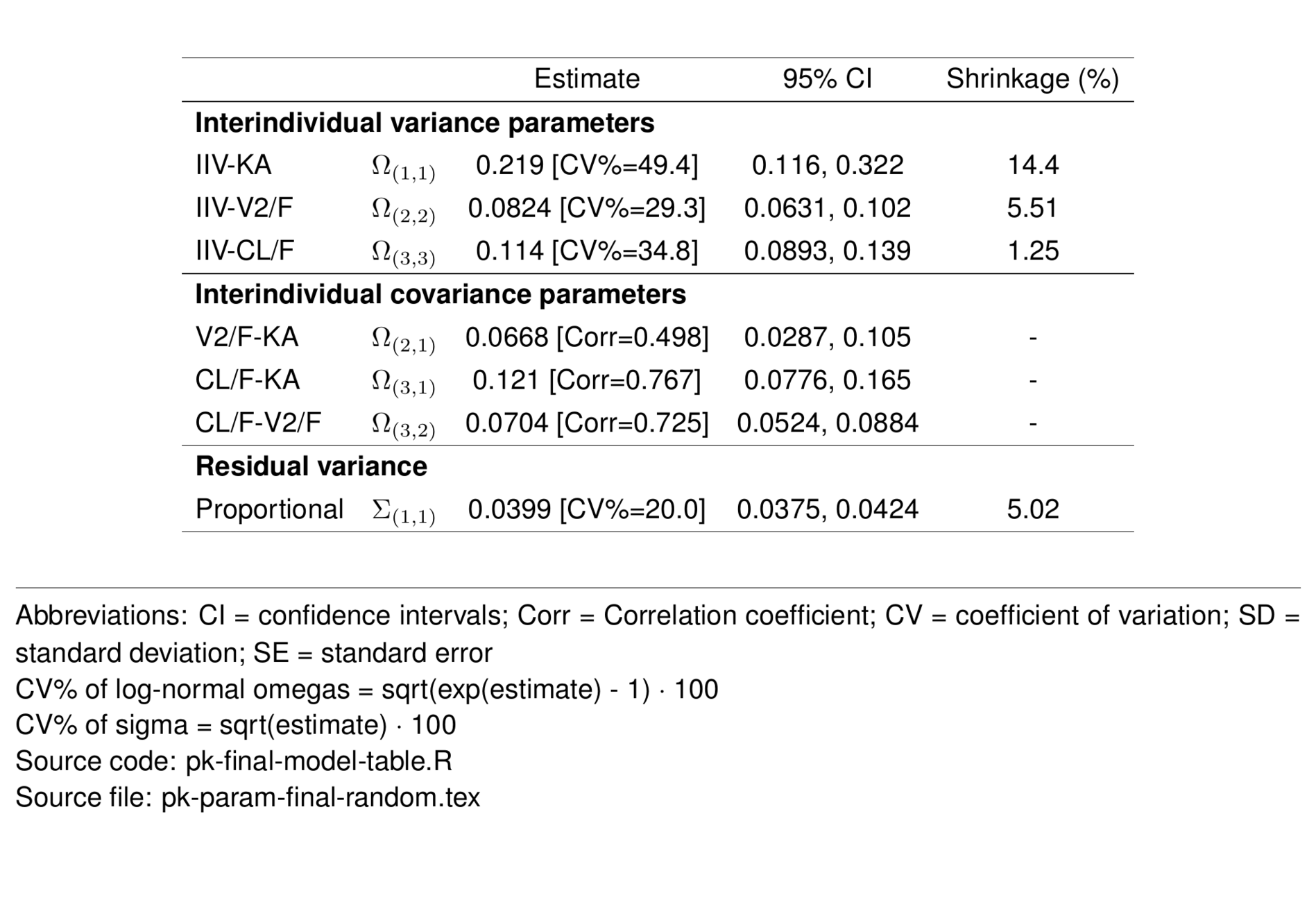
6 Create bootstrap parameter table
The bootstrap parameter table process works similarly to the final model parameter table above, but includes a few additional steps that are specific to a bootstrap run.
6.1 Bootstrap parameters
The bootstrap estimates are read in, summarized, and joined to the parameter key:
define_boot_tableCombines bootstrap estimates with non-bootstrap estimates and parameter key Performs some formatting of this combined data frame.- reads in the bootstrap model output generated in Bootstrap Generate and Collect.
- uses
bbr::param_estimates_compareto extract summary quantiles, the 5th, 50th and 95th, of the bootstrap estimates for each model parameter. These quantiles can be updated as needed. - renames the columns for the parameter table.
- removes punctuation in the parameter name column (needed to join it to the parameter key).
- joins parameter details from the parameter key.
format_boot_tableFormats bootstrap parameter estimate values and output selected columns to be shown in the bootstrap parameter table.- selects columns for final tables. Default selects “abb”, “desc”, “boot_value”, “boot_ci_95”. To return all columns, specify “all” for .select_cols.
boot <- readr::read_csv(here("data/boot/boot-106.csv"))


boot_df = boot %>%
  define_boot_table(.nonboot_estimates = sum,
                    .key = pathKey) %>%
  format_boot_table()
6.2 Final model parameters
After manipulating the bootstrap run parameters, we join them with the final model parameter table param_df.
Note that this parameter table includes the 95% CI directly from the bootstrap results (and not the estimated interval calculated from the final model).
bootParam = left_join(param_df, boot_df, by = c("abb", "desc"))6.3 Create tex versions of the parameter tables
As mentioned above, our reports are written in Latex, so we now convert the param_df to two Latex report-ready tex tables using the pmtables package: one table for fixed effects and one table for random effects.
6.3.1 Fixed effect parameter table
bootfixed = bootParam %>%
  filter(str_detect(type, "Struct") |
           str_detect(type, "effect")) %>%
  select(-shrinkage, -ci_95) %>%
  st_new() %>%
  st_panel("type") %>%
  st_span("Final model", value) %>%
  st_span("Non-parametric bootstrap", boot_value:boot_ci_95) %>%
  st_center(desc = col_ragged(5.5),
            abb = "l") %>%
  st_blank("abb", "greek", "desc") %>%
  st_rename("Estimate" = "value",
            "Median" = "boot_value",
            "95\\% CI" = "boot_ci_95") %>%
  st_files(output = "pk-param-boot-fixed.tex") %>%
  st_notes("Parameters estimated in the log-domain were
           back transformed for clarity") %>%
  st_notes(glue("The confidence interval was determined from the
                      2.5th and 97.5th percentiles of the non-parametric
                      bootstrap (n={nrow(boot)}) estimates.")) %>%
  st_notes("Abbreviations: CI = confidence interval") %>%
  st_noteconf(type = "minipage", width = 1) %>%
  stable() %>%
  stable_save()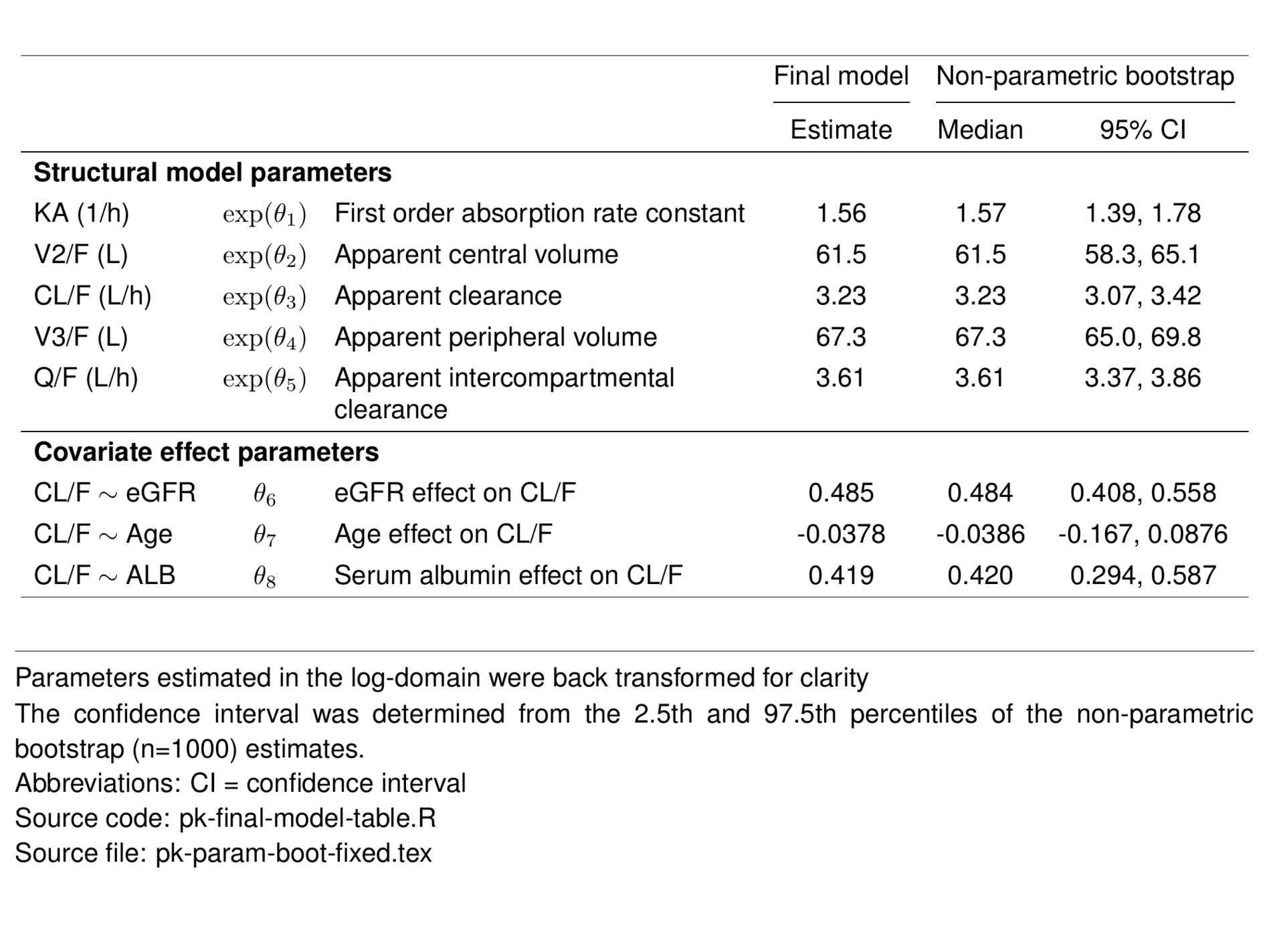
6.3.2 Random effects parameter table
bootrandom = bootParam %>%
  filter(stringr::str_detect(greek, "Omega") |
           str_detect(type, "Resid")) %>%
  select(-desc, -ci_95)  %>%
  st_new %>%
  st_panel("type") %>%
  st_span("Final model", value:shrinkage) %>%
  st_span("Non-parametric bootstrap", boot_value:boot_ci_95) %>%
  st_center(abb = "l") %>%
  st_blank("abb", "greek") %>%
  st_rename("Estimate" = "value",
            "Median" = "boot_value",
            "95\\% CI" = "boot_ci_95",
            "Shrinkage (\\%)" = "shrinkage") %>%
  st_files(output = "pk-param-boot-random.tex") %>%
  st_notes(glue("The confidence interval was determined from the
                      2.5th and 97.5th percentiles of the non-parametric
                      bootstrap (n={nrow(boot)}) estimates.")) %>%
  st_notes("Abbreviations: CI = confidence interval;
                        Corr = correlation coefficient;
                        CV = coefficient of variation") %>%
  st_notes("CV\\% of log-normal omegas = sqrt(exp(estimate) - 1) $\\cdot$ 100") %>%
  st_notes("CV\\% of sigma = sqrt(estimate) $\\cdot$ 100") %>%
  st_noteconf(type = "minipage", width = 1) %>%
  stable() %>%
  stable_save()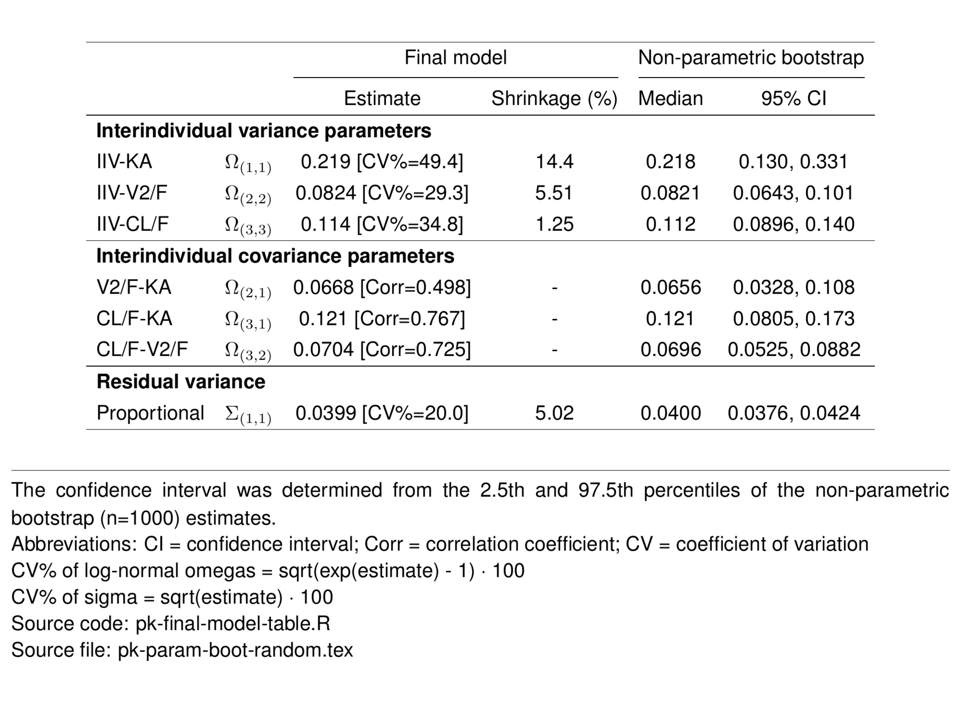
7 Other resources
More detail about the creating parameter tables with pmparams can be found in its published Vignettes.