1 Introduction

The pmforest package can be used to visualize the covariates of interest in your analysis by creating grouped displays of point estimates and variability ranges for any kind of continuous data.

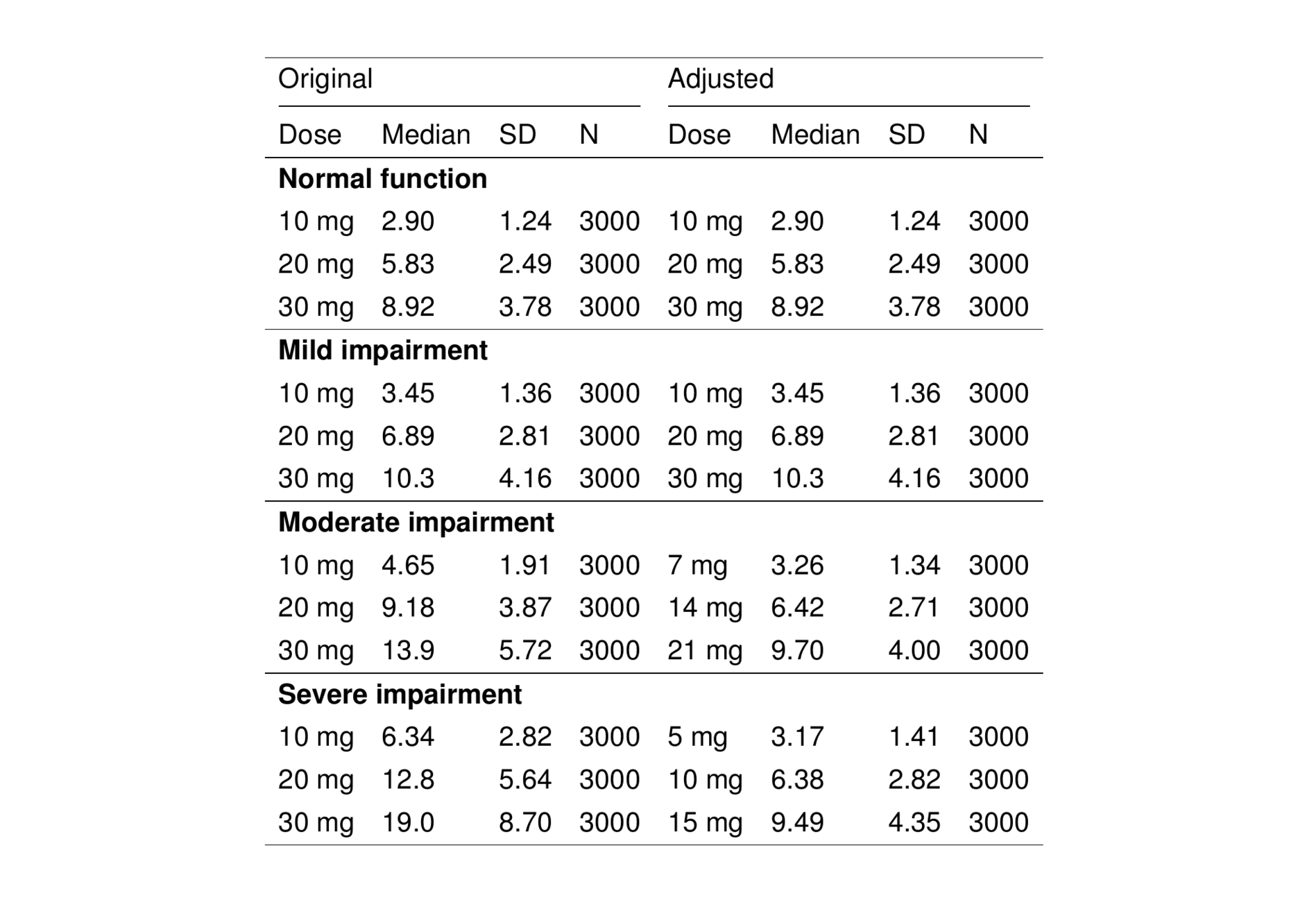
2 Example data

To illustrate this package, we created some example data looking at dose adjustments for renal impairment. Here we’ve calculated AUCss at different doses for subjects with varying levels of renal function.

head(data)

   ID             RFf dosef     type       CL      AUC
1:  1 Normal function 10 mg original 2.536364 3.942651
2:  2 Normal function 10 mg original 1.555193 6.430070
3:  3 Normal function 10 mg original 2.579118 3.877295

In one set of simulations, a standard set of doses were evaluated regardless of renal function (Original) while another simulation set implemented a simple dose adjustment scheme for subjects with moderate or severe renal impairment (Adjusted).

Figure 1: AUCss for different levels of renal function simulated for original or adjusted doses.

3 Forest plots

To display the central tendency and variability in these data graphically using the pmforest package we follow a two-step procedure.

3.1 Step 1: summarize the data

We call summarize_data() to create data summaries that will be plotted.

adjusted <- filter(data, type=="adjusted")

summ1 <- summarize_data(
  data = adjusted, 
  value = "AUC", 
  group = "RFf", 
  group_level = "dosef"
)

This function provided by pmforest creates a summary data frame that is in the correct format for processing by plot_forest() in the next step.

head(summ1)

# A tibble: 6 × 5
  group           group_level   mid    lo    hi
  <fct>           <fct>       <dbl> <dbl> <dbl>
1 Normal function 10 mg        2.90  1.56  5.49
2 Normal function 20 mg        5.83  3.13 11.0 
3 Normal function 30 mg        8.92  4.62 16.6 
4 Mild impairment 10 mg        3.45  1.85  6.16
5 Mild impairment 20 mg        6.89  3.72 12.9 
6 Mild impairment 30 mg       10.3   5.62 18.7

3.2 Step 2: create the forest plot

We create a plot of the summarized data using plot_forest(), passing in the summarized data and some additional settings.

plot_forest(
  summ1, 
  vline_intercept = NULL, 
  x_lab = "AUCss (ng*hr/mL)", 
  x_limit = c(0, 41)
)

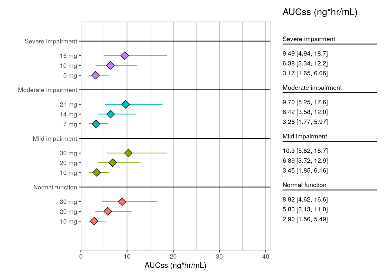
Figure 2: AUCss simulated under simple dose-adjustment scheme.

In the summarized data, the group column sets the outer grouping in the plot (renal function level) and the group_level column sets the levels within that grouping factor (in this case, the doses).

Also, note that the summary metrics are by default:

mid: the median
lo: the 5th percentile
hi: the 95th percentile

All these summaries are customizable from the summarize_data() function.

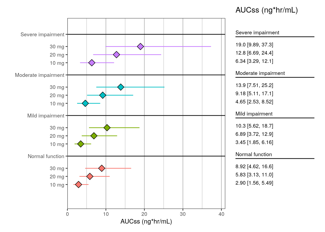
We can make a similar plot for the original dosing scenario.

original <- filter(data, type=="original")

summ2 <- summarize_data(
  data = original, 
  value = "AUC", 
  group = "RFf", 
  group_level = "dosef"
)

head(summ2)

# A tibble: 6 × 5
  group           group_level   mid    lo    hi
  <fct>           <fct>       <dbl> <dbl> <dbl>
1 Normal function 10 mg        2.90  1.56  5.49
2 Normal function 20 mg        5.83  3.13 11.0 
3 Normal function 30 mg        8.92  4.62 16.6 
4 Mild impairment 10 mg        3.45  1.85  6.16
5 Mild impairment 20 mg        6.89  3.72 12.9 
6 Mild impairment 30 mg       10.3   5.62 18.7

plot_forest(
  summ2, 
  vline_intercept = NULL, 
  x_lab = "AUCss (ng*hr/mL)", 
  x_limit = c(0, 41)
)

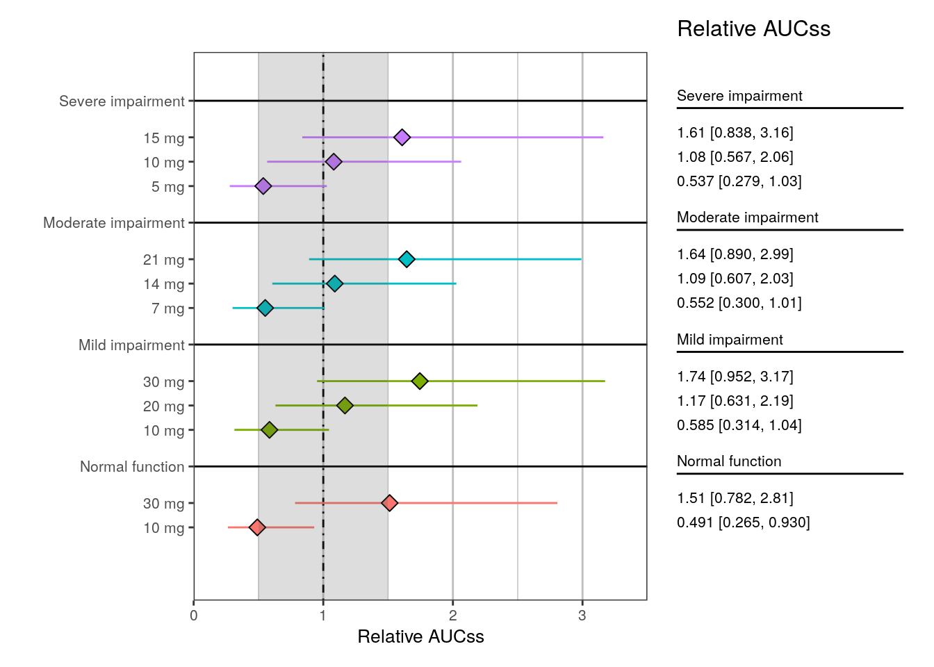
Figure 3: AUCss simulated under original dose set.

3.3 Mark a region of interest

We can also annotate a region of interest or equivalence on the x-axis.

summ4 <- summarize_data(
  data = adjusted, 
  value = "AUCrel", 
  group = "RFf", 
  group_level = "dosef"
)

plot_forest(
  summ4, 
  vline_intercept = 1, 
  x_lab = "Relative AUCss", 
  x_limit = c(0, 3.5), 
  shaded_interval = c(0.5, 1.5),
  shape_size = 3
)

Figure 4: Relative AUCss simulated under the dose adjustment set.