library(tidyverse)
library(yaml)
library(yspec)
library(pmplots)
library(mrggsave)
library(mrgmisc)
library(here)
library(data.table)1 Introduction
During the exploratory data analysis (EDA) phase of a project, we typically create a series of plots (and tables) to better understand our data. This page walks through
- Creating a selection of these plots using the
pmplotsorggplot2packages. See Introduction to pmplots for more information. - Using the information in your data specification (spec) file, and the
yspecpackage, to easily subset data, decode categorical data and annotate plots. See the Introduction to yspec for more information. - Using
mrggsaveto save plots to a predefined figure directory.
2 Tools used
2.1 MetrumRG packages
yspec Data specification, wrangling, and documentation for pharmacometrics.
pmplots Create exploratory and diagnostic plots for pharmacometrics.
mrggsave Label, arrange, and save annotated plots and figures.
2.2 CRAN packages
dplyr A grammar of data manipulation.
3 Outline
The pk.csv data set used in these examples is in data/derived/ and has an accompanying spec file, pk.yml.
Before continuing, it’s important you’re familiar with the following terms to understand the examples below:
- yspec: refers to the package.
- spec file: refers to the data specification yaml describing your data set.
- spec object: refers to the R object created from your spec file and used in your R code.
More information on these terms is given on the Introduction to yspec page.
Below we create:
- Continuous covariate pairs plots
- Boxplots of continuous versus categorical covariates
- Various grouped concentration-time plots
- Concentration-time plots per individual
4 Set up
4.1 Required packages
4.2 Other set up
Set your global mrggsave options.
options(mrg.script = "eda-figures.R", mrggsave.dir = figDir)4.3 Load your analysis ready data set
dat = fread(file = here("data", "derived", "pk.csv"), na.strings = '.')5 Extracting information from your spec file
5.1 Load your spec file
Load your spec file as a spec object.
spec = ys_load(here("data", "derived", "pk.yml"))5.2 Namespace options
Look at the available namespaces and select your preferred namespace.
ys_namespace(spec)
specTex = ys_namespace(spec, "tex")

head(specTex, 5)
name info unit short source
1 C cd- . Commented rows lookup
2 NUM --- . Row number lookup
3 ID --- . NONMEM ID number lookup
4 TIME --- hour Time after first dose lookup
5 SEQ -d- . Data type lookup5.3 Filter your spec object
Use the information in the spec file to filter the data to the covariates of interest using flags.
contCovDF = ys_filter(spec, covariate)
contCovNames = names(contCovDF)

head(contCovDF, 5)
name info unit short source
1 AGE --- years Age lookup
2 WT --- kg Weight lookup
3 EGFR --- mL/min/1.73m2 Estimated GFR lookup
4 ALB --- g/dL Albumin lookup5.4 Axes labels
Generate and customize the axes labels for your covariate plots. Here we use the short label (in the tex namespace) if it’s under 10 characters long and convert the short label to title case. We also manually update the facet labels for EGFR to put the units on a new line.
contCovarListTex = axis_col_labs(specTex,
                                 contCovNames,
                                 title_case = TRUE,
                                 short = 10)

contCovarListTex["EGFR"] = "EGFR//EGFR \n(ml/min/1.73m^2)"

head(contCovarListTex, 5)
AGE WT
"AGE//Age (years)" "WT//Weight (kg)"
EGFR ALB
"EGFR//EGFR \n(ml/min/1.73m^2)" "ALB//Albumin (g/dL)" 5.5 Decode numerical categorical variables
Categorical covariates often need to be coded numerically for modeling purposes. You can use the decode information in your yspec to convert these numerical columns to factors with levels and labels that match the decode descriptions.
We also create a new DoseNorm variable that we’ll use later to plot the dose-normalized concentration over time.
dat2 = dat %>%
  yspec_add_factors(spec, STUDY, CP, RF, DOSE) %>%
  mutate(DoseNorm = DV/DOSE)

head(dat2 %>% distinct(ID, DOSE, DOSE_f))
ID DOSE DOSE_f
<int> <int> <fctr>
1: 1 5 5 mg
2: 2 5 5 mg
3: 3 5 5 mg
4: 4 5 5 mg
5: 5 5 5 mg
6: 6 10 10 mg6 Extracting individual covariate data
To create plots of the baseline covariate values we need to do some data grooming to extract one row per patient for all covariates of interest.
covar = dat2 %>%
  distinct(ID, .keep_all = TRUE) %>%
  rename(Study = STUDY_f) %>%
  select(ID, AMT, AGE:ALB, LDOS, STUDY, RF,
         CP,  Study:DoseNorm, NUM)
7 Continuous covariate pairs plot
Plot the relationship between continuous covariates using the pairs_plot function, a wrapper to GGally::ggpairs(). Use the columns and labels extracted from the spec object in contCovarListTex to automatically rename the panel labels.
ContVCont = covar %>%
  pairs_plot(y = contCovarListTex) +
  rot_x(50)
ContVCont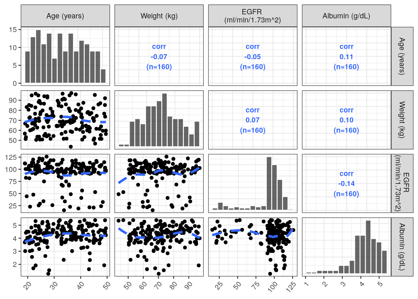
7.1 Save plot to a pdf
mrggsave(ContVCont,
         stem = "cont-vs-cont",
         width = 6, height = 7)
8 Boxplots of continuous versus categorical covariates
8.1 Continuous versus categorical boxplots for the total population
Plot the continuous covariates (extracted in contCovarListTex) versus each categorical covariate using wrap_cont_cat. This function makes the data set long with respect to the contCovarListTex variables, facets the rendered plot and automatically renames the facets using the information extracted from the spec file.
renal_contCat_Total = covar %>%
  wrap_cont_cat(x = "RF_f//Renal Function Group",
                y = contCovarListTex,
                use_labels = TRUE
  ) + rot_x(35)
renal_contCat_Total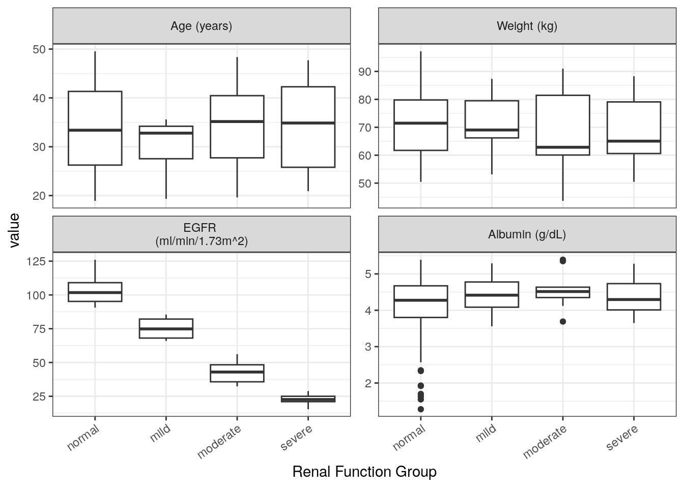
8.2 Continuous versus categorical boxplots; stratified by study
Plot each continuous covariate (extracted in contCovarListTex) versus the categorical covariates of interest and facet by study. We show one covariate plot as an example but the code returns a named list of plots.
renal_contCat_Study = map(contCovarListTex, function(.y){
  cont_cat(df = covar, x = 'RF_f//Renal Function Group', y = .y) +
    facet_wrap(~STUDY, labeller = label_both) +
    rot_x(35)
})renal_contCat_Study$AGE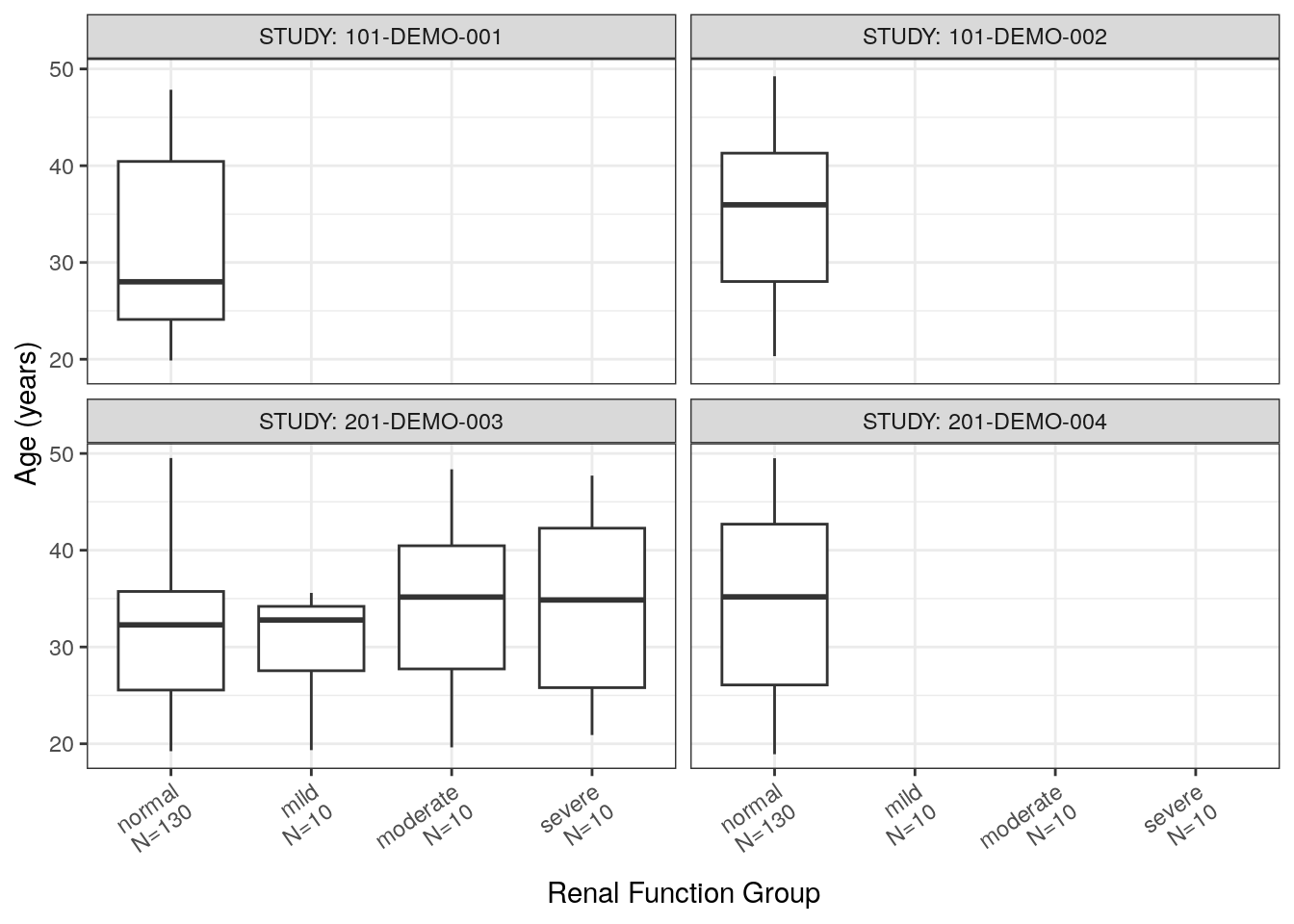
8.3 Save list of plots into one pdf
mrggsave(list(renal_contCat_Total, renal_contCat_Study),
         stem = "cat-vs-cont")
9 Concentration-time plots
9.1 Set up
Filter the data set to include only the pharmacokinetic (PK) observations above the limit of quantification and define the x- and y-axis labels.
dat3 = dat2 %>% filter(EVID==0, BLQ==0)

xLabT = 'Time (h)'
xLabTAD = 'Time after dose (h)'
yLab = 'Concentration (ng/mL)'
yLabNorm = 'Dose-normalized concentration (ng/mL*mg)'
9.2 Helper functions
9.2.1 Set color palette for plots
.plot_color_theme = function(...) {
  scale_color_brewer(..., palette = "Set1")
}
9.2.2 Filter data for plotting
Plots were created only for the time periods of interest. In this case
- after the first dose,
- after the last dose, and
- over the full time course for each study
The filter_df arguments include:
df= dataframe to be filteredstudy= name of study to filter data set on (defaults to NULL)tlo= lower bound to filter TIME on (defaults to -inf)thi= upper bound to filter TIME on (defaults to inf)tadlo= lower bound to filter TAD on (defaults to -inf)tadhi= upper bound to filter TAD on (defaults to inf)
filter_df = function(df,
                     study = NULL,
                     tlo = -Inf,
                     thi = Inf,
                     tadlo = -Inf,
                     tadhi = Inf) {
  df = df %>% filter(TIME >= tlo & TIME <= thi)
  df = df %>% filter(TAD >= tadlo & TAD <= tadhi)
  if (!is.null(study)) df = df %>% filter(STUDY_f == study)
  return(df)
}
9.2.3 Plot concentration
plot_Conc arguments:
.df= dataframe for plotting.logy= put y-axis on a log scale (expects TRUE/FALSE).by_group= column name of the grouping variable for facet wrap.color= column name to use for coloring of data in plots.group= column name to use for grouping data in plots.legendName= name for legend items.x= column to be used on x axis (default = TIME).y= column to be used on y axis (default = DV).xLab= label for x-axis (default = xLabT).yLab= label for y-axis (default = yLab).incLine= define whether line should be included forgroupargument (expects TRUE/FALSE).smooth= define whether to include smooth LOESS line (expects TRUE/FALSE)
plot_Conc = function(.df,
                     .logy = FALSE,
                     .by_group = NULL,
                     .color = NULL,
                     .group = NULL,
                     .legendName = NULL,
                     .x = TIME,
                     .y = DV,
                     .xLab = xLabT,
                     .yLab = yLab,
                     .incLine = TRUE,
                     .smooth = FALSE) {

  p = ggplot(data = .df, aes(x = {{.x}}, y = {{.y}})) +
    geom_point(aes(color = {{.color}})) +
    labs(x = .xLab, y = .yLab, colour = NULL)  +
    .plot_color_theme(name = .legendName) +
    pm_theme()
  if(.incLine){
    p = p + geom_line(aes(color = {{.color}}, group = {{.group}}))
  }
  if(.smooth){
    p = p + geom_smooth(aes(color = {{.color}}, group = {{.group}}),
                        method = 'loess', formula = 'y ~ x')
  }
  if (!is.null(.by_group)) {
    p = p + facet_wrap( ~.data[[.by_group]], scales = "free", ncol = 2)
  }
  if (.logy) {
    p = p + scale_y_log10()
  }
  p
}
9.3 Concentration time profiles
We include Study 101-DEMO-001 and plots of the first 24 hours post-dose (other examples are given in the full script).
df01 =  dat3 %>%
        filter_df(thi = 24, study = '101-DEMO-001')
9.3.1 Concentration versus time
This example uses the default options of the plot_Conc function: concentration (i.e., the dependent variable, DV) versus time. It includes options:
.colorthe data by dose group..groupby ID, i.e., include a line connecting each individuals observations in the plot.- Use
.logyto put the y-axis on a log-scale. - Use
.legendNameto rename the title of the legend.
MET1 = plot_Conc(.df=df01, .color=DOSE_f, .group=ID,
                 .logy=TRUE, .legendName="Dose Group")
MET1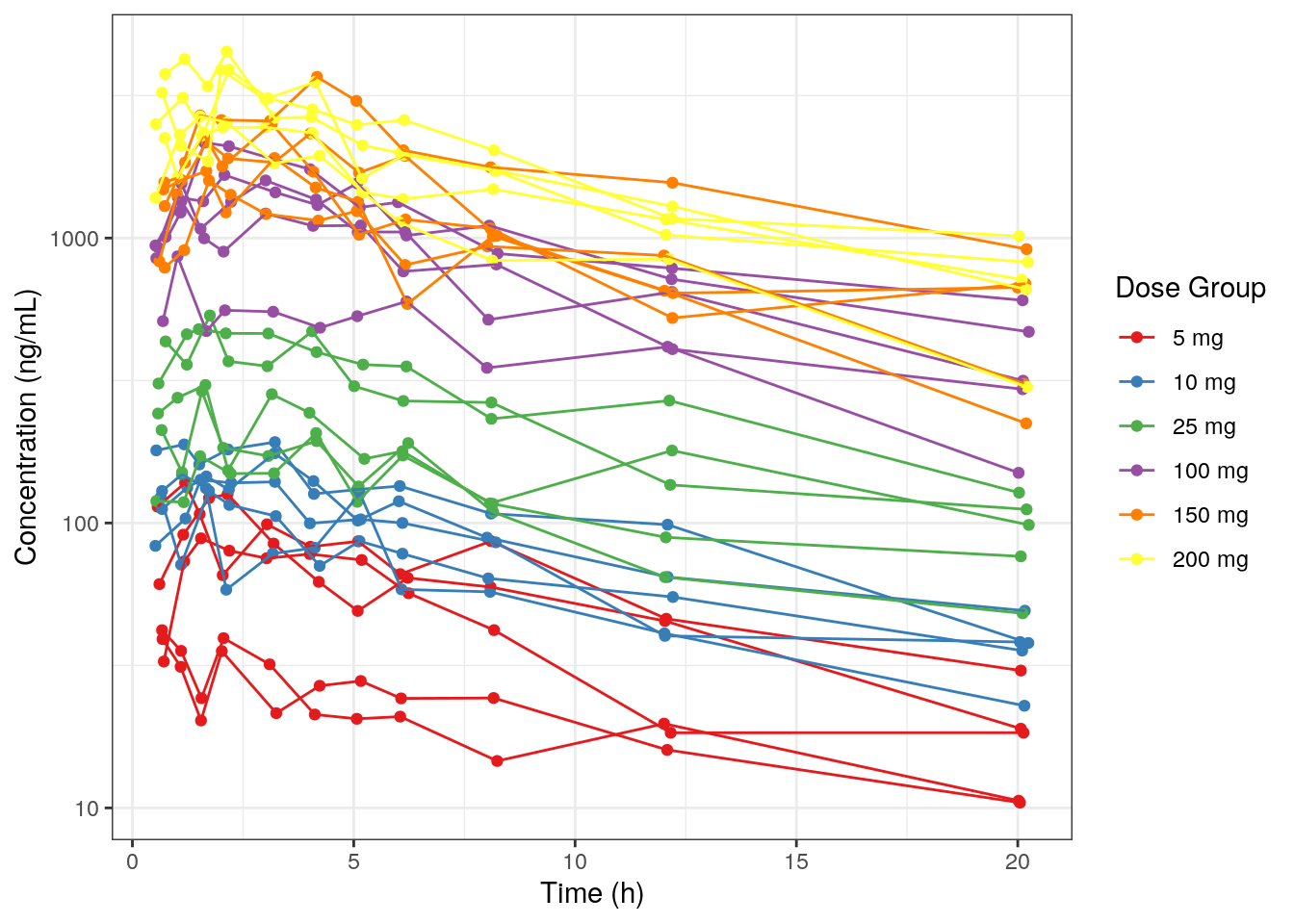
9.3.2 Dose-normalized concentration versus time
Create a plot of dose-normalized concentration versus time by:
- changing the y-axis variable
.yto the dose-normalized concentration column, DoseNorm. - changing the y-axis label with
.yLab.
MET1a = plot_Conc(.df=df01, .y=DoseNorm, .yLab = yLabNorm,
                  .logy=TRUE, .legendName="Dose Group",
                  .color=DOSE_f, .group=ID)
MET1a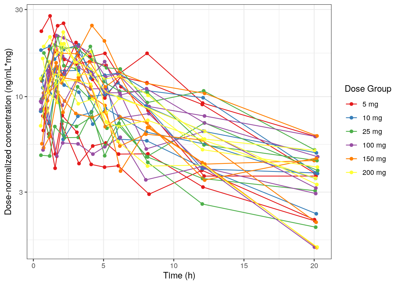
9.3.3 Concentration versus time with smooth LOESS line by dose
- Use
.groupto group data by dose group such that there is a line for each dose group in the plot. - Add smooth LOESS line with
.smooth - Suppress outputting a line between dose groups with
.incline.
MET1b = plot_Conc(.df=df01, .color=DOSE_f, .group=DOSE_f,
                  .logy=TRUE, .legendName="Dose Group",
                  .incLine = F, .smooth = TRUE)
MET1b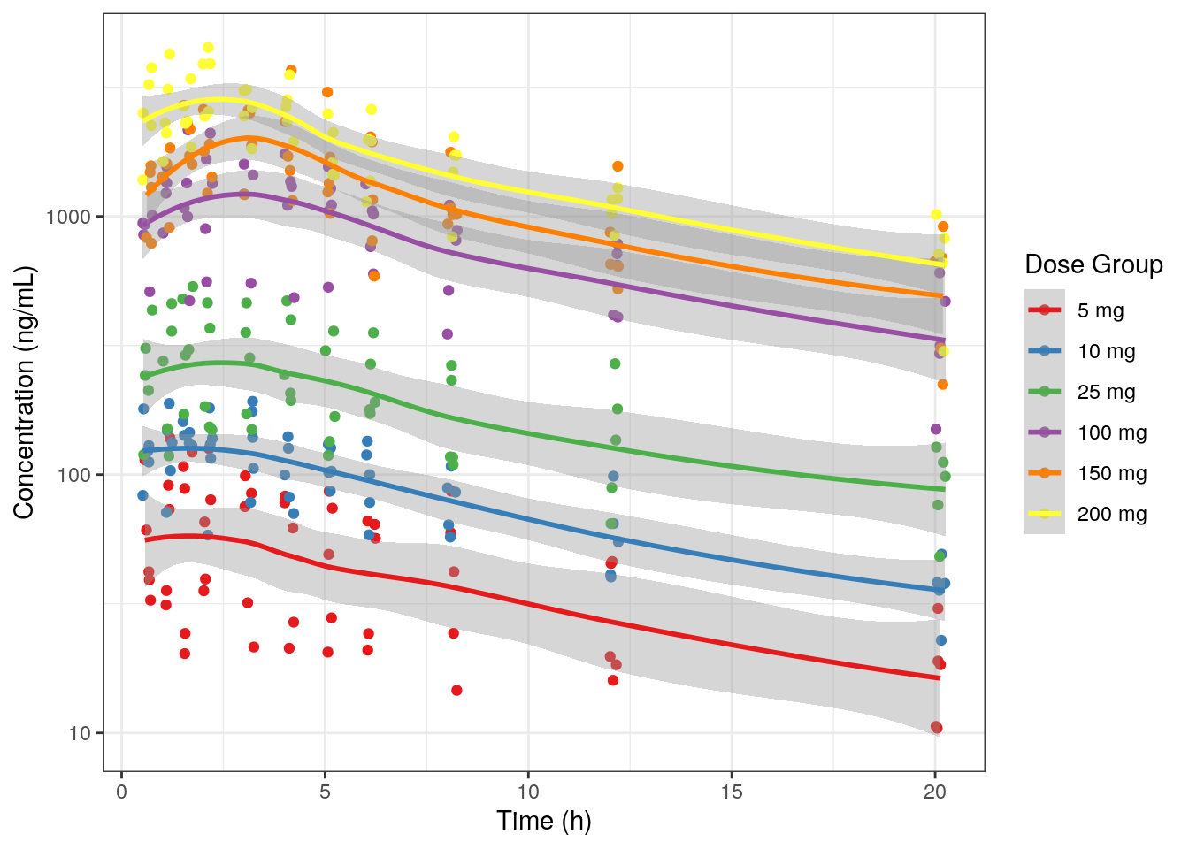
9.3.4 Concentration versus time after dose (TAD)
- Use
.xto change the x-axis to TAD (default=TIME) - Update the x-axis label with
.yLab - Use
.groupto group data by ID such that there is a line for each ID in the plot
MET1_tad = plot_Conc(.df=df01, .color =DOSE_f, .group =ID,
                     .logy=TRUE, .legendName="Dose Group",
                     .x=TAD, .xLab = xLabTAD)
MET1_tad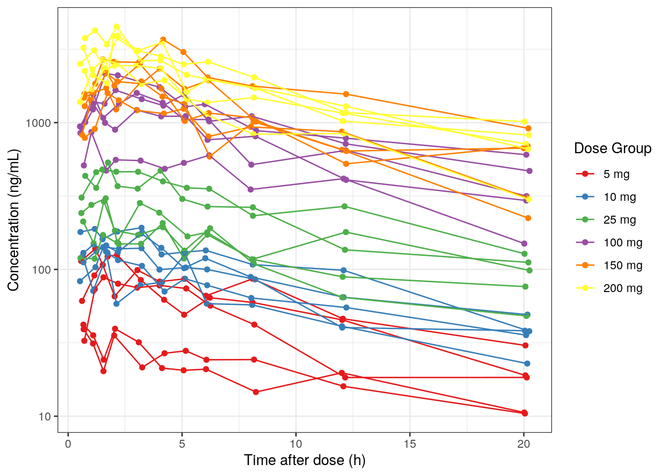
9.4 Save a list of plots to one pdf
mrggsave(list(MET1,MET1a,MET1b,MET1_tad),
         stem = "pk-plots", width = 6)
9.5 Save each plot separately as pngs
mrggsave(list(MET1,MET1a,MET1b,MET1_tad),
          tag = "pk-plots",
          onefile=FALSE,
          dev = "png",
          width=5, height=5)
10 Concentration-time plots per ID
Use the mrgmisc package to split your data set and create a series of plots faceted by individual. In this example, we create individual plots of concentration over time with a vertical dashed grey line to indicate reported dose times. Update the ids_per_plot function to modify the number of individuals/facets per plot.
split_Obs = dat2 %>% filter(EVID==0) %>%
  mutate(ID = asNum(ID)) %>%
  mutate(PLOTS = ids_per_plot(ID, 4)) %>% # default is 9 per subplot
  split(.[["PLOTS"]])

split_Dose = dat2 %>% filter(EVID==1) %>%
  mutate(ID = asNum(ID)) %>%
  mutate(PLOTS = ids_per_plot(ID, 4)) %>% # default is 9 per subplot
  split(.[["PLOTS"]])

#This function can/should be edited to address project specific questions
p_conc_time = function(dfO, dfD) {
  ggplot() +
    geom_point(data=dfO, aes(x=TIME, y=DV)) +
    geom_line(data=dfO, aes(x=TIME, y=DV, group=ID)) +
    # dashed vertical line to indicate dose times
    geom_vline(data=dfD, aes(xintercept=TIME),
               linetype="dashed", colour="grey") +
    facet_wrap(~STUDY+ID, scales= "free") +
    pm_theme() + theme(legend.position = "none") +
    labs(x = xLabT, y = yLab)
}

IDplotList = map2(split_Obs, split_Dose, p_conc_time) IDplotList$`9`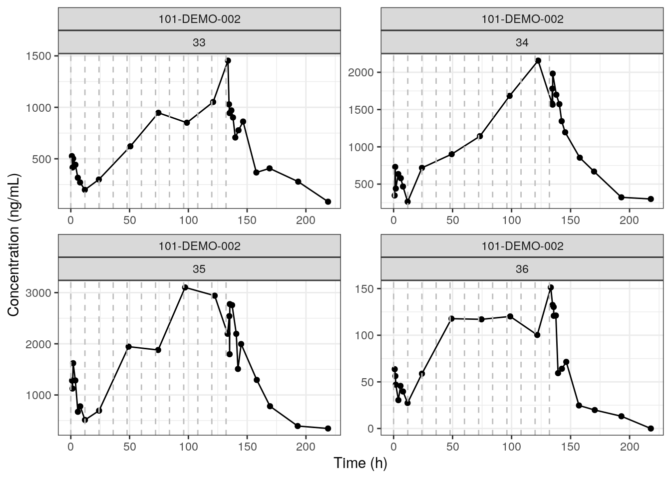
The rendered plot is PK concentration over time of Study 101-DEMO-002 for 4 IDs. We chose this study with multiple doses to showcase the reported dose time dashed lines.
10.1 Save a list of plots to one pdf
mrggsave(IDplotList, stem = "id-dose-dv")