library(tidyverse)
library(pmtables)
library(yspec)
library(here)
library(magrittr)
library(data.table)1 Introduction
During the exploratory data analysis (EDA) phase of a project, we typically create a series of tables (and plots) to better understand our data. This page walks through
- Creating a selection of these tables using the
pmtablespackage. - Using the information in your data specification (spec) file, and the
yspecpackage, to easily subset data, decode categorical data and annotate tables. - Summarizing your data with
pmtablesfunctions.
2 Tools used
2.1 MetrumRG packages
yspec Data specification, wrangling, and documentation for pharmacometrics.
pmtables Create summary tables commonly used in pharmacometrics and turn any R table into a highly customized tex table.
2.2 CRAN packages
dplyr A grammar of data manipulation.
3 Outline
The pk.csv data set used in these examples is in data/derived/ and has an accompanying spec file, pk.yml.
Before continuing, it’s important you’re familiar with the following terms to understand the examples below:
- yspec: refers to the package.
- spec file: refers to the data specification yaml describing your data set.
- spec object: refers to the R object created from your spec file and used in your R code.
More information on these terms is given on the Introduction to yspec page.
Below we create the following tables:
- Data inventory tables including the number (%) of subjects, observations and below limit of quantification (BLQ) data per study; total and by dose group
- Categorical covariate summaries stratified by study, dose group and renal function or Child-Pugh score
- Continuous covariate summaries stratified by study, renal function or Child-Pugh score
Both the categorical and continuous summary tables provide prespecified summary statistics. However, users can pass a function to replace this default, allowing totally customized summaries. Please see the pmtables User book for more details on this and other features beyond the scope of this page.
4 Set up
4.1 Required packages
4.2 Other set up
# set up directories
scriptDir = here("script")
tabDir = tempdir()

set.seed(5238974)

# set script name (for table annotation) and table directory location
options(mrg.script = "eda-tables.R", pmtables.dir = tabDir)

## Helper function to return a numeric variable
asNum  = function(f){ return(as.numeric(as.character(f))) }
4.3 Load the analysis ready data set
dat <- fread(file = here("data", "derived", "pk.csv"),
             na.strings = '.')
5 Extracting information from your spec file
5.1 Load your spec file
Load your spec file as a spec object.
spec <- ys_load(here("data", "derived", "pk.yml"))5.2 Namespace options
Useys_namespace to view the available namespaces. Specify the tex namespace with specTex = ys_namespace(spec, "tex").
ys_namespace(spec)
specTex <- ys_namespace(spec, "tex")
head(specTex, 5)
. name info unit short source
. 1 C cd- . Commented rows lookup
. 2 NUM --- . Row number lookup
. 3 ID --- . NONMEM ID number lookup
. 4 TIME --- hour Time after first dose lookup
. 5 SEQ -d- . Data type lookup5.3 Extract data from your spec object
Extract the units for each column of your dataset from your spec object.
units <- ys_get_unit(specTex, parens = TRUE)
units$TIME
. [1] "(hour)"Generate covariate labels using the short and units fields of your spec object. This function includes several options, including putting any units in parentheses or automatically converting the short label to title case.
covlab <- ys_get_short_unit(specTex, parens = TRUE, title_case = TRUE)
head(covlab, 5)
. $C
. [1] "Commented Rows"
.
. $NUM
. [1] "Row Number"
.
. $ID
. [1] "NONMEM ID Number"
.
. $TIME
. [1] "Time after First Dose (hour)"
.
. $SEQ
. [1] "Data Type"5.4 Make empty list for tables
While this step is not essential, we find it helpful to add all tables to a named list as we create them. This is particularly useful if you want to create a pdf preview file for all your tables (or a subset of tables) at the end of the script. Here we open a blank list.
tableList <- list()6 Data inventory table
The pt_data_inventory function counts the number of subjects and observations in your dataset. These counts can be stratified (or panelled) by categorical covariates, for example, counts by study or disease status. The function returns the number (and percent) of observations that are above the limit of quantification, below the limit of quantification (BLQ) or missing.
6.1 Decode numerical categorical variables
Categorical covariates often need to be coded numerically for modeling purposes. You can use the decode information in your spec object to convert these numerical columns to factors with levels and labels that match the decode descriptions.
pkSum <- dat %>%
  yspec_add_factors(spec, STUDY, CP, RF, DOSE, SEQ) %>%
  filter(is.na(C), SEQ==1)

head(pkSum %>% distinct(ID, DOSE, DOSE_f))
. ID DOSE DOSE_f
. <int> <int> <fctr>
. 1: 1 5 5 mg
. 2: 2 5 5 mg
. 3: 3 5 5 mg
. 4: 4 5 5 mg
. 5: 5 5 5 mg
. 6: 6 10 10 mgThe pmtables summary functions assume the user has subset their data to only the records to be included in the summary, for example, here we summarize the pkSum dataset that includes only the observation records (SEQ = 1).
6.2 Number and percent of subjects, observations and BLQ per study
Use the pt_data_inventory function to count the number of subjects and observations in your dataset and panel the summary by study. Assign the output file name and saved it out as a tex file.
tab <- pkSum %>%
  pt_data_inventory(by = c("Study" = "STUDY_f")) %>%
  st_new() %>%
  st_files(output = "pk-data-sum.tex") %>%
  stable() %>%
  stable_save()

tableList$`pk-data-sum` <- tab
st_as_image(tab)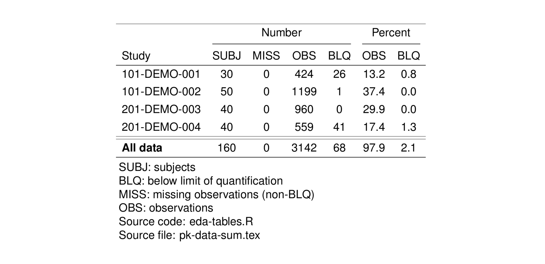
Use st2report() to check how your table looks in our report template.
tableList$'pk-data-sum' %>% st2report() 7 Categorical covariate summary table
Categorical data can be summarized in either a wide or long format. Here we demonstrate how to use pt_cat_wide to summarize categorical data in a wide format. The summary is number (percent within group) and, in this example, counts the number (and percent) of subjects within each renal function category, stratified by study and dose group.
tab <- pkSum %>%
  distinct(ID, DOSE_f, STUDY_f, RF_f, .keep_all = TRUE) %>%
  pt_cat_wide(
    cols = c("Renal function" = "RF_f"),
    panel = as.panel("STUDY_f", prefix = "Study:"),
    by = c("Dose Group" = "DOSE_f")
  ) %>%
  stable(output_file =  "rf-per-dose.tex") %>%
  stable_save()
tableList$'rf-per-dose' <- tab
st_as_image(tab)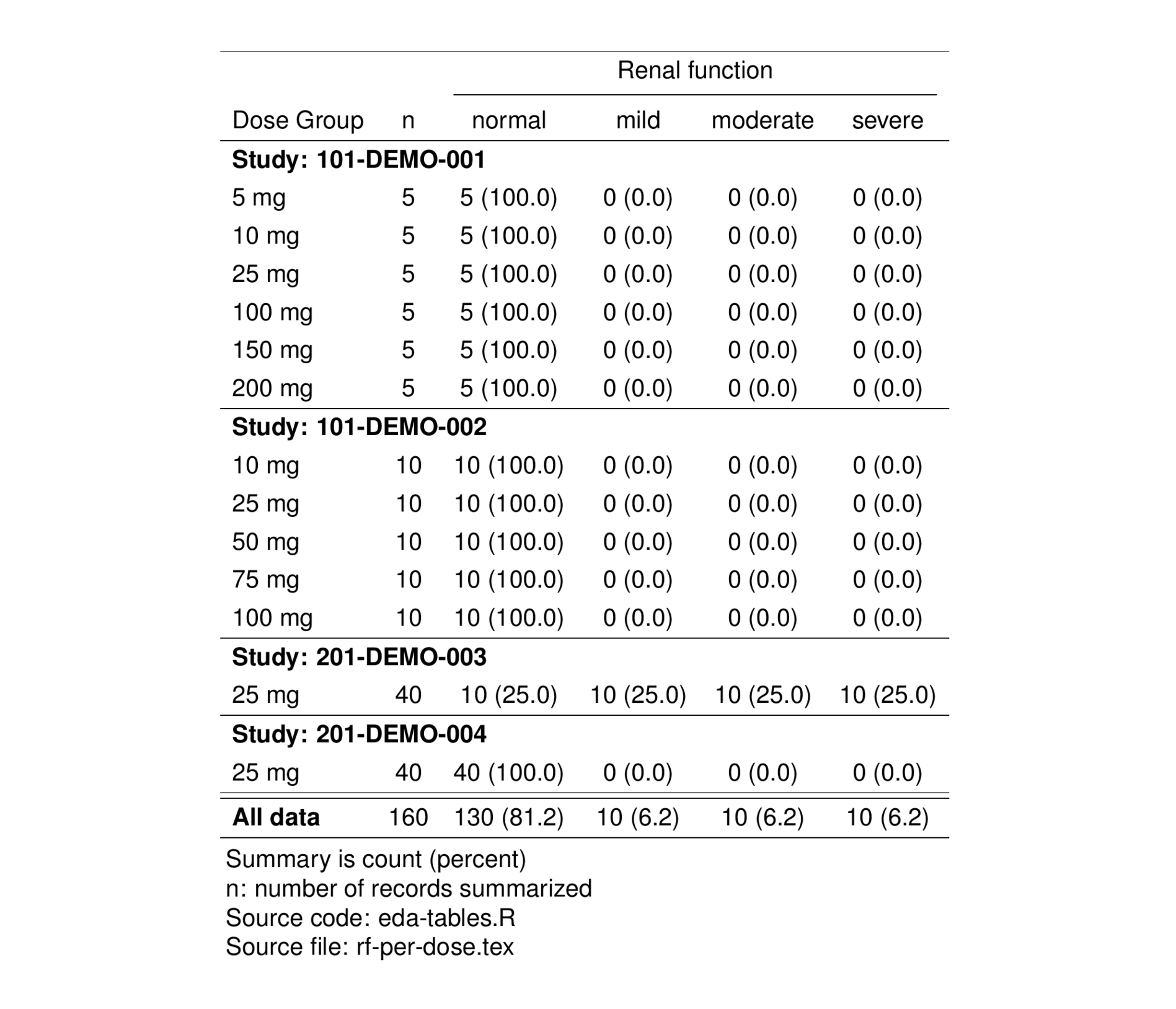
8 Continuous covariate summary table
Continuous data can be summarized in either a wide or long format. Here we show how to use pt_cont_long to summarize continuous covariates in a long format (i.e., covariates go down the table). These tables can be stratified (or panelled) by categorical covariates, for example, counts by study or disease status.
8.1 Set up
Use yspec_add_factors to decode information in your spec object to convert categorical covariates to factors with levels. Select the variables of interest.
covID <- dat %>%
  yspec_add_factors(spec, STUDY, CP, RF, SEQ) %>%
  yspec_add_factors(spec, DOSE, .suffix = "") %>%
  filter(is.na(C)) %>%
  select(ID:TIME, AGE:CP, PHASE:SEQ_f)

head(covID)
. ID TIME AGE WT HT EGFR ALB BMI SEX AAG SCR AST
. <int> <num> <num> <num> <num> <num> <num> <num> <int> <num> <num> <num>
. 1: 1 0.00 28.03 55.16 159.55 114.45 4.4 21.67 1 106.36 1.14 11.88
. 2: 1 0.61 28.03 55.16 159.55 114.45 4.4 21.67 1 106.36 1.14 11.88
. 3: 1 1.15 28.03 55.16 159.55 114.45 4.4 21.67 1 106.36 1.14 11.88
. 4: 1 1.73 28.03 55.16 159.55 114.45 4.4 21.67 1 106.36 1.14 11.88
. 5: 1 2.15 28.03 55.16 159.55 114.45 4.4 21.67 1 106.36 1.14 11.88
. 6: 1 3.19 28.03 55.16 159.55 114.45 4.4 21.67 1 106.36 1.14 11.88
. ALT CP PHASE STUDYN DOSE SUBJ USUBJID STUDY
. <num> <int> <int> <int> <fctr> <int> <char> <char>
. 1: 12.66 0 1 1 5 mg 1 101-DEMO-0010001 101-DEMO-001
. 2: 12.66 0 1 1 5 mg 1 101-DEMO-0010001 101-DEMO-001
. 3: 12.66 0 1 1 5 mg 1 101-DEMO-0010001 101-DEMO-001
. 4: 12.66 0 1 1 5 mg 1 101-DEMO-0010001 101-DEMO-001
. 5: 12.66 0 1 1 5 mg 1 101-DEMO-0010001 101-DEMO-001
. 6: 12.66 0 1 1 5 mg 1 101-DEMO-0010001 101-DEMO-001
. ACTARM RF STUDY_f CP_f RF_f SEQ_f
. <char> <char> <fctr> <fctr> <fctr> <fctr>
. 1: DEMO 5 mg norm 101-DEMO-001 normal normal Dose
. 2: DEMO 5 mg norm 101-DEMO-001 normal normal Observation
. 3: DEMO 5 mg norm 101-DEMO-001 normal normal Observation
. 4: DEMO 5 mg norm 101-DEMO-001 normal normal Observation
. 5: DEMO 5 mg norm 101-DEMO-001 normal normal Observation
. 6: DEMO 5 mg norm 101-DEMO-001 normal normal ObservationExtract one row per patient.
timeIndCoDF <- distinct(covID, ID, .keep_all = TRUE)8.2 Filter your spec object
Use ys_get_short_unit to extract the abbreviations from the spec object for the table footer. Then, use the information in the spec file to filter the data set to the covariates of interest using flags.
labs <- ys_get_short_unit(specTex, parens = TRUE)
contCovDF <- ys_filter(specTex, covariate)

head(contCovDF)
. name info unit short source
. 1 AGE --- years Age lookup
. 2 WT --- kg Weight lookup
. 3 EGFR --- mL/min/1.73m$^2$ Estimated GFR lookup
. 4 ALB --- g/dL Albumin lookup8.3 Continous covariate summary by study
Use pt_cont_long to summarize continuous covariates in a long format (i.e., covariates go down the table). The default summary statistics include a count (n), the mean, median, standard deviation, minimum, and maximum for the covariates of interest. Here we also summarized by study and for all data.
tab <- timeIndCoDF %>%
  pt_cont_long(
    cols = names(contCovDF),
    panel = as.panel("STUDY_f", prefix = "Study:"),
    table = covlab
  ) %>%
  st_new() %>%
  st_files(output = "cont-covar-sum.tex") %>%
  st_notes_detach(width = 1) %>%
  st_notes_str() %>%
  stable() %>%
  stable_save()

tableList$'cont-covar-sum' <- tab

st_as_image(tab)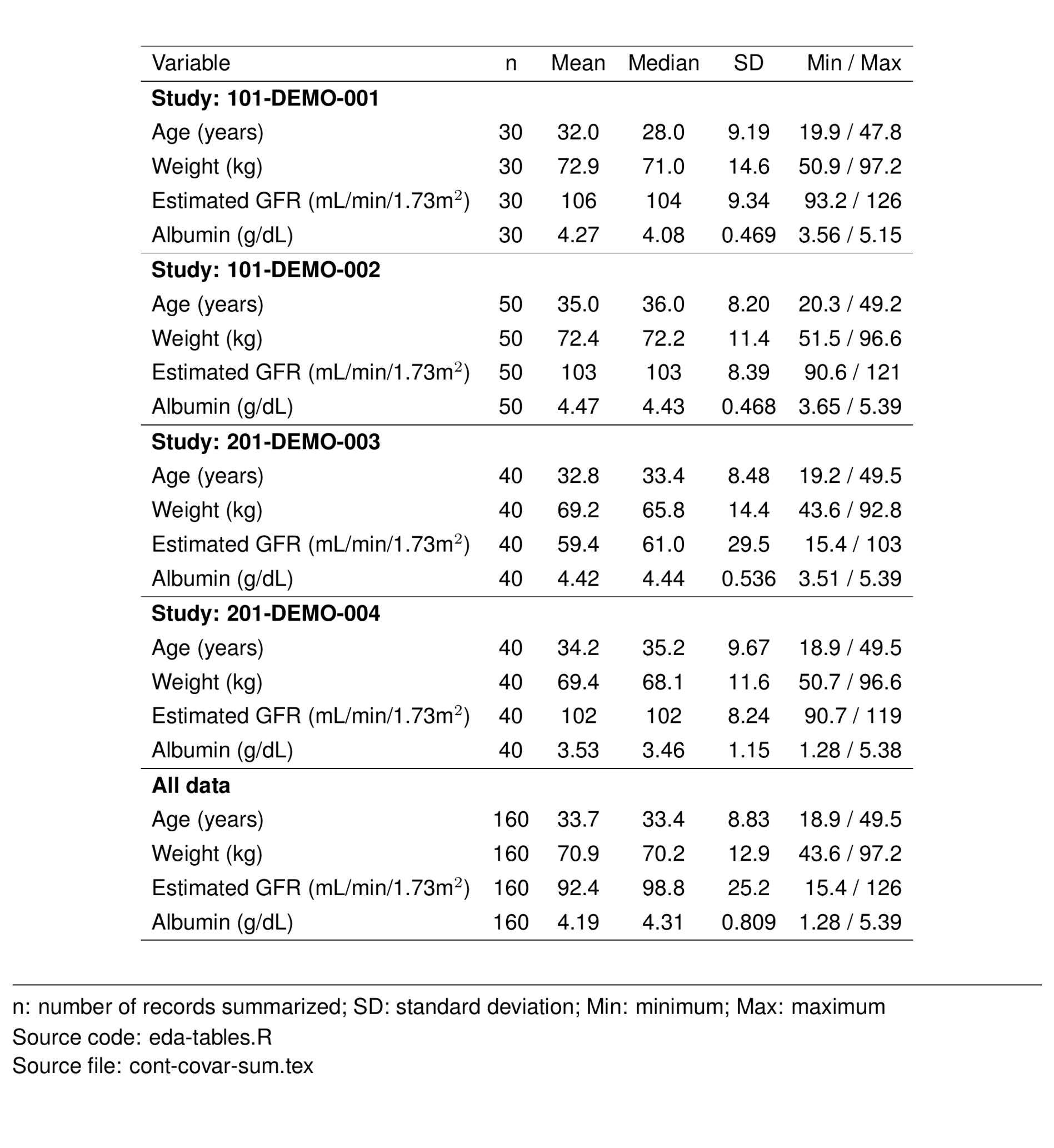
9 Preview tables in the report template
While these functions typically save out tex versions of the tables for use in our Latex reports, we also preview how these tables look with our report template, e.g., to check the tables fit within the report margins. This preview can also be saved out as a pdf.
if(interactive()) {
  st2report(
    tableList,
    ntex = 2,
    stem = "preview-eda", ## name of pdf preview
    output_dir = tabDir
  )
}