106.The final covariate model included the following features:
Two compartment disposition parameterized in terms of:
First-order absorption (KA)
First-order elimination
Allometric scaling- clearances and volumes
Covariate effects
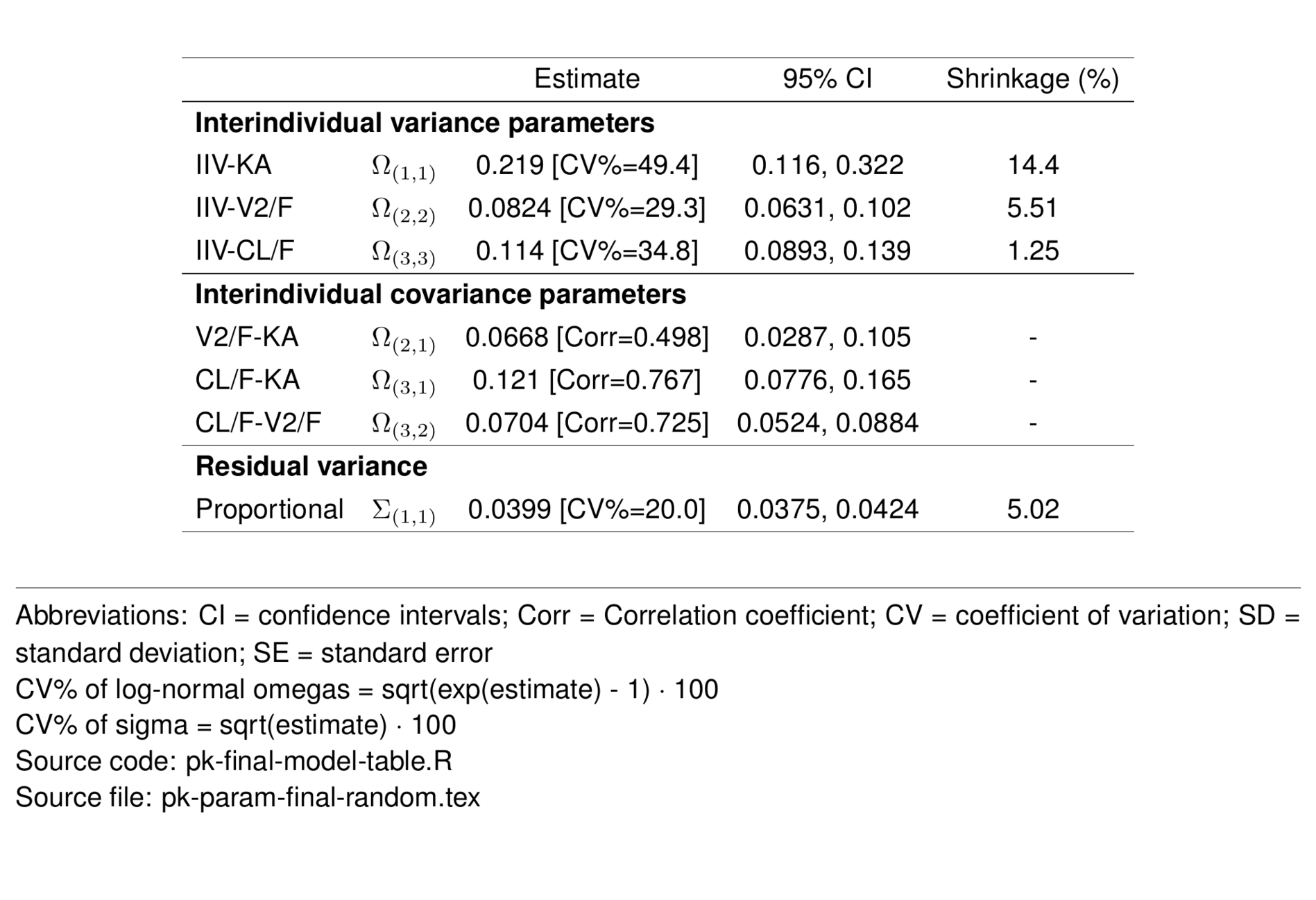
Subject-level random effects
Proportional residual error
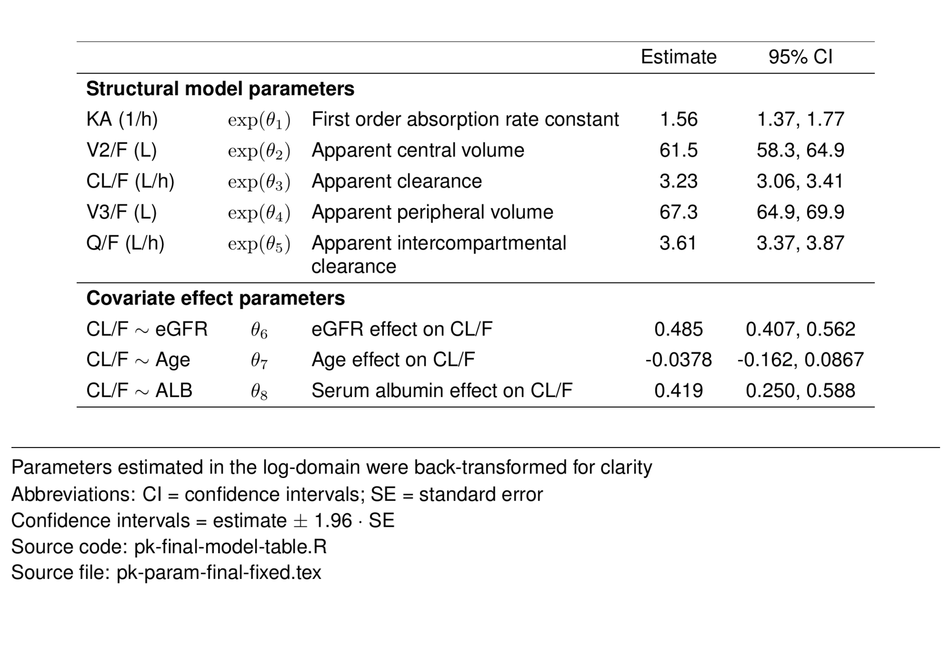
The final model included fixed effects of body weight on all CL/F and V/F terms. Additionally, the effects of age, eGFR and albumin were estimated on drug CL/F.
\[ CL/F_i = e^{(\theta_{3} + \text{WT}_\mathit{CL/F} + \text{EGFR}_\mathit{CL/F} + \text{AGE}_\mathit{CL/F} + \text{ALB}_\mathit{CL/F} + \eta_{3i})} \]
\[ \mathit{V2/F_i}=e^{(\theta_{2} + \text{WT}_{V/F} + \eta_{2i})} \\ \] \[ \mathit{Q/F_i}=e^{(\theta_{5} + \text{WT}_{Q/F})} \] \[ \mathit{V3/F_i}=e^{(\theta_{4} + \text{WT}_{V/F})} \]
\[ \mathit{KA_i}=e^{(\theta_{1} + \eta_{1i})} \\ \]
where
\[ \text{WT}_\mathit{CL/F} = 0.75 \cdot \log\big(\text{WT}_i/70\big) \]
\[ \text{EGFR}_\mathit{CL/F} = \theta_6 \cdot \log\big(\text{EGFR}_i/90\big) \]
\[ \text{AGE}_\mathit{CL/F} = \theta_7 \cdot \log\big(\text{AGE}_i/35\big) \]
\[ \text{ALB}_\mathit{CL/F} = \theta_8 \cdot \log\big(\text{ALB}_i/4.5\big) \]
\[ \text{WT}_\mathit{V/F} = 1.00 \cdot \log\big(\text{WT}_i/70\big) \]
\[ \text{WT}_\mathit{Q/F} = 0.75 \cdot \log\big(\text{WT}_i/70\big) \]
\[ Y_\mathit{i,y} = \widehat{Y_\mathit{i,j}} \cdot \big(1+\varepsilon_\mathit{i,j}\big) \]
where
106.
106.library(mrgsolve)
library(dplyr)
library(here)
library(ggplot2)
library(forcats)
library(patchwork)
theme_set(theme_bw())
mod <- mread(here("script/model/106.mod")) %>% zero_re()
data <- as_data_set(
evd(amt = 25),
evd(amt = 25, ii = 24, addl = 10)
)
out <- mrgsim(mod, data, output = "df", delta = 0.1, end = 480)
out <- mutate(
out,
lbl = case_when(
ID==1 ~ "Single dose",
ID==2 ~ "Multiple dose, q24h x10"
),
lbl = forcats::fct_inorder(lbl)
)
b <- filter(out, ID==2)
a <- filter(out, ID==1 & TIME <= 96)
pa <- ggplot(a) +
geom_line(aes(TIME, Y)) +
facet_wrap(~lbl, scales = "free_x") +
labs(x = "Time (hours)", y = "Concentration (ng/mL)") +
scale_x_continuous(breaks = seq(0,96,8)) +
scale_y_continuous(limits = c(0, 600))
pb <-
ggplot(b) +
geom_line(aes(TIME/24, Y)) +
facet_wrap(~lbl, scales = "free_x") +
labs(x = "Time (days)", y = "") +
scale_x_continuous(breaks = seq(0,20,2)) +
scale_y_continuous(limits = c(0, 600))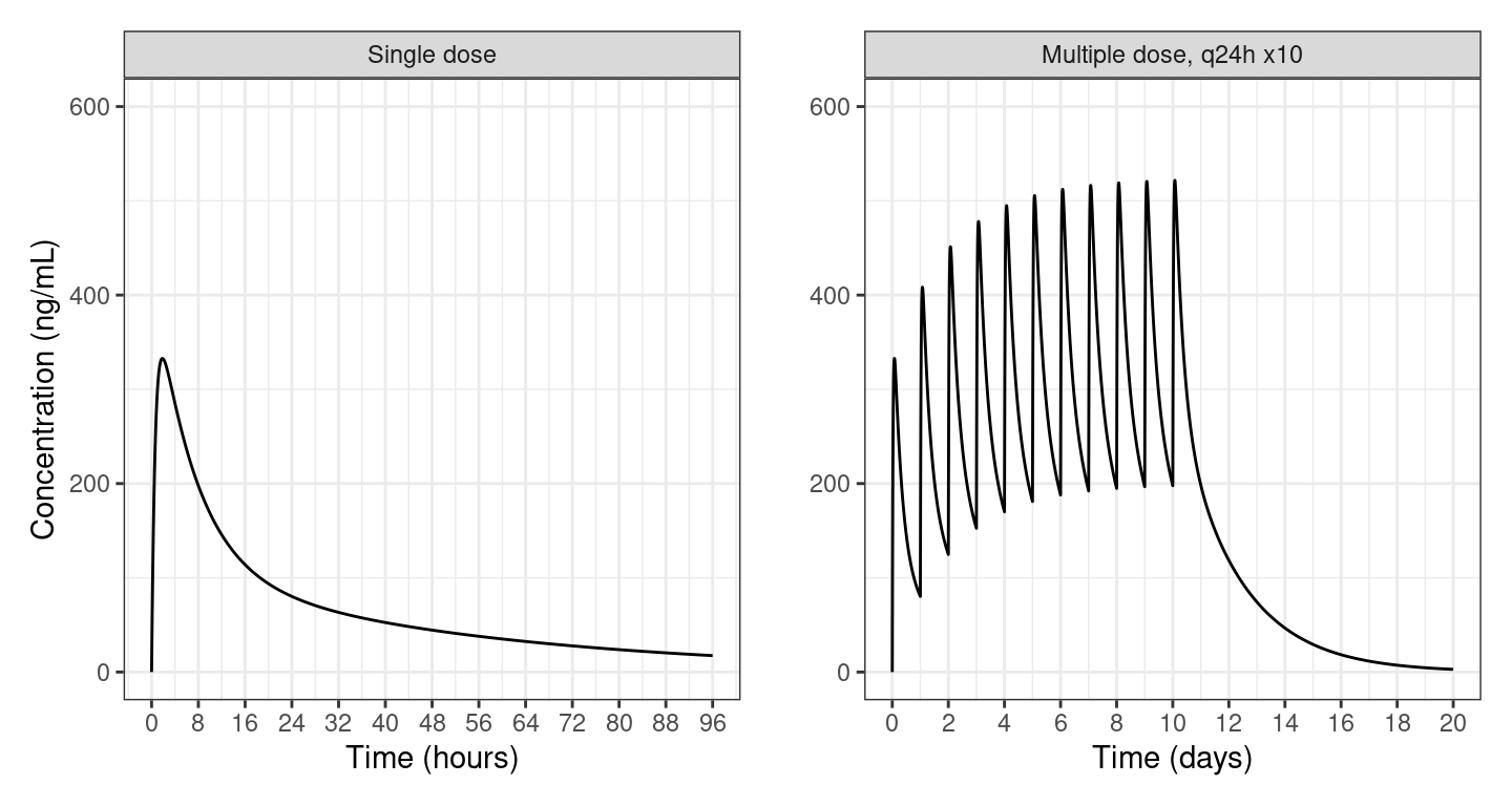
$PROBLEM From bbr: see 106.yaml for details

$INPUT C NUM ID TIME SEQ CMT EVID AMT DV AGE WT HT EGFR ALB BMI SEX AAG
       SCR AST ALT CP TAFD TAD LDOS MDV BLQ PHASE

$DATA ../../../data/derived/pk.csv IGNORE=(C='C', BLQ=1)

$SUBROUTINE ADVAN4 TRANS4

$PK

;log transformed PK parms

V2WT = LOG(WT/70)
CLWT = LOG(WT/70)*0.75
CLEGFR = LOG(EGFR/90)*THETA(6)
CLAGE = LOG(AGE/35)*THETA(7)
V3WT = LOG(WT/70)
QWT  = LOG(WT/70)*0.75
CLALB = LOG(ALB/4.5)*THETA(8)


KA   = EXP(THETA(1)+ETA(1))
V2   = EXP(THETA(2)+V2WT+ETA(2))
CL   = EXP(THETA(3)+CLWT+CLEGFR+CLAGE+CLALB+ETA(3))
V3   = EXP(THETA(4)+V3WT)
Q    = EXP(THETA(5)+QWT)

S2 = V2/1000 ; dose in mcg, conc in mcg/mL

$ERROR
IPRED = F
Y=IPRED*(1+EPS(1))

$THETA  ; log values
(0.5)   ;  1 KA (1/hr) - 1.5
(3.5)   ;  2 V2 (L) - 60
(1)     ;  3 CL (L/hr) - 3.5
(4)     ;  4 V3 (L) - 70
(2)     ;  5 Q  (L/hr) - 4
(1)     ;  6 CLEGFR~CL ()
(1)     ;  7 AGE~CL ()
(0.5)   ;  8 ALB~CL ()

$OMEGA BLOCK(3)
0.2   ;ETA(KA)
0.01 0.2   ;ETA(V2)
0.01 0.01 0.2   ;ETA(CL)

$SIGMA
0.05     ; 1 pro error

$EST MAXEVAL=9999 METHOD=1 INTER SIGL=6 NSIG=3 PRINT=1 RANMETHOD=P MSFO=./106.MSF
$COV PRINT=E RANMETHOD=P
$TABLE NUM IPRED NPDE CWRES CL V2 Q V3 KA ETAS(1:LAST) NOPRINT ONEHEADER RANMETHOD=P FILE=106.tab[ prob ]
106-104 + COV-effects(CRCL, AGE) on CL
This model requires mrgsolve >= 1.0.3
[ plugin ] autodec nm-vars
[ pkmodel ] cmt = "GUT,CENT,PERIPH", depot = TRUE
[ input ]
WT = 70
EGFR = 90
ALB = 4.5
AGE = 35
DOSE = 25
[ nmxml ]
path = "../../model/pk/106/106.xml"
root = "cppfile"
[ pk ]
V2WT = LOG(WT/70.0);
CLWT = LOG(WT/70.0)*0.75;
CLEGFR = LOG(EGFR/90.0)*THETA(6);
CLAGE = LOG(AGE/35.0)*THETA(7);
V3WT = LOG(WT/70.0);
QWT = LOG(WT/70.0)*0.75;
CLALB = LOG(ALB/4.5)*THETA(8);
KA = EXP(THETA(1) + ETA(1));
V2 = EXP(THETA(2) + V2WT + ETA(2));
CL = EXP(THETA(3) + CLWT + CLEGFR + CLAGE + CLALB + ETA(3));
V3 = EXP(THETA(4) + V3WT);
Q = EXP(THETA(5) + QWT);
S2 = V2/1000.0; //; dose in mcg, conc in mcg/mL
[ error ]
IPRED = CENT/S2;
Y = IPRED * (1+EPS(1));
capture AUC = DOSE/CL;
[ capture ] CL V2 IPRED Y