1 Introduction

During model development goodness-of-fit (GOF) diagnostic plots are generated to assess model fit. Here we demonstrate how to generate diagnostic plots for models using the pmplots and yspec packages. For more information on which diagnostics are most appropriate for your project and how to interpret them please refer to the Other resources section at the bottom of this page.

After working through how to create the diagnostic plots on this page we recommend looking at the Parameterized Reports for Model Diagnostics page. There we show how you can put this code into an R Markdown template and use a feature of R Markdown, the “parameterized report”, to generate a series of diagnostic plots. The idea is that you might create one or two templates during the course of your project and then render each template from the single model-diagnostics.R script to generate diagnostic plots for multiple models.

2 Tools used

2.1 MetrumRG packages

yspec Data specification, wrangling, and documentation for pharmacometrics.

pmplots Create exploratory and diagnostic plots for pharmacometrics.

bbr Manage, track, and report modeling activities, through simple R objects, with a user-friendly interface between R and NONMEM®.

2.2 CRAN packages

dplyr A grammar of data manipulation.

mrgmisc Format, manipulate and summarize data in the field of pharmacometrics.

3 Outline

Our model diagnostics are made using the pmplots package and leveraging the information provided in the spec file through the yspec package functions.

Below we demonstrate how to read in your NONMEM® output and create the following plots:

Observed vs predicted diagnostic plots
Normalized prediction distribution error (NPDE) diagnostic plots
Conditional weighted residuals (CWRES) diagnostic plots
Empirical Bayes estimate(EBE)-based diagnostic plots

This is obviously not an exhaustive list and, while we make diagnostics for the final model, run 106, this code can be used for all models. The pk.csv data set was created in the data assembly script (da-pk-01.Rmd) and has an accompanying data specification (spec), pk.yml, in the data/spec directory.

Before continuing, it’s important you’re familiar with the following terms to understand the examples below:

yspec: refers to the package.
spec file: refers to the data specification yaml describing your data set.
spec object: refers to the R object created from your spec file and used in your R code.

More information on these terms is given on the Introduction to yspec page.

4 Set up

4.1 Required packages

library(bbr)
library(dplyr)
library(pmplots)
library(here)
library(yspec)
library(glue)
library(patchwork)

library(mrgmisc)
library(yaml)
library(knitr)
library(pmtables)

4.2 Other set up

Code for general set up

### Helper functions
source(here('script/functions-diagnostics.R'))

5 Extracting information from your spec file

5.1 Load your spec file

spec <- ys_load(here("data","derived","pk.yml"))
head(spec)

   name info  unit                 short source
1     C  cd-     .        Commented rows lookup
2   NUM  ---     .            Row number lookup
3    ID  ---     .      NONMEM ID number lookup
4  TIME  ---  hour Time after first dose lookup
5   SEQ  -d-     .             Data type lookup
6   CMT  -d-     .           Compartment lookup
7  EVID  -d-     .      Event identifier lookup
8   AMT  ---    mg           Dose amount lookup
9    DV  ---     .    Dependent variable lookup
10  AGE  --- years                   Age lookup

5.2 Namespace options

Useys_namespace to view the available namespaces - here we’re going to use the plot namespace.

ys_namespace(spec)

namespaces:

 - base
 - long
 - plot
 - tex

spec <- ys_namespace(spec, "plot")

5.3 Extract data from your spec object

The covariates of interest for your diagnostic plots could be defined explicitly in the code, for example,

diagContCov <- c("AGE","WT","ALB","EGFR")
diagCatCov <- c("STUDY", "RF", "CP", "DOSE")

Alternatively, you can define the covariates of interest once in your spec file using flags and simply read them in here

diagContCov <- pull_meta(spec, "flags")$diagContCov
diagCatCov <- pull_meta(spec, "flags")$diagCatCov

Learn about yspec flags

A flags argument is used to extract only specific columns from the spec object.

When creating a spec file, you can specify flags in the SETUP section. The variables in the covariate section of flags will then be selected when using ys_filter(spec, covariate).
Alternatively, if you chose not to use flags, you can use ys_select to select variables by name, e.g., ys_select(spec, c(AGE, WT, EGFR, ALB)).

6 Read in the model output

6.1 Model Object

We use read_model from the bbr package to read the model details into R and assign it to a mod object.

This mod object can be piped to other functions in the bbr package to further understand the model output, for example, by passing the mod object to the model_summary function you can see

the analysis dataset location
the number of records, observations and subjects included
the objective function and estimation method(s)
a summary of any heuristic problems detected
a table of the model parameter estimates, standard errors and shrinkage

mod <- read_model(here("model","pk","106"))
sum <- mod %>% model_summary()

6.2 Model dataset

All our NONMEM®-ready datasets include a row number column (a unique row identifier typically called NUM) that’s added during data assembly. And, when running NONMEM® models, we always request this NUM column in each $TABLE. This allows us to take advantage of a bbr function called nm_join that reads in all output table files and joins them back to the input data set.

data0 <- nm_join(mod)

The idea is that in NONMEM®, you table just NUM and no other input data items because these all get joined back to the nonmem output (including the character columns) by nm_join.

By default, the input data is joined to the table files so that the number of rows in the result will match the number of rows in the table files (i.e., the number of rows not bypassed via $IGNORE statements). Use the .superset argument to join table outputs to the (complete) input data set.

The plot data should include the observation records only (i.e., EVID==0) and we use the decode information in your spec object, with the yspec_add_factors function, to convert the numerical columns to factors with levels and labels that match the decode descriptions for the plot labels.

data <- 
  data0 %>% 
  filter(EVID==0) %>% 
  yspec_add_factors(spec, .suffix = "")

7 General diagnostic plots

7.1 Observed vs predicted plots

Observed (DV) vs predicted (PRED or IPRED) plots can be created easily using the dv_pred and dv_ipred functions in pmplots. These functions include several options to customize your plots, including using more specific names (shown below).

dvp <- dv_pred(data, yname = "concentration (mg/L)")
dvp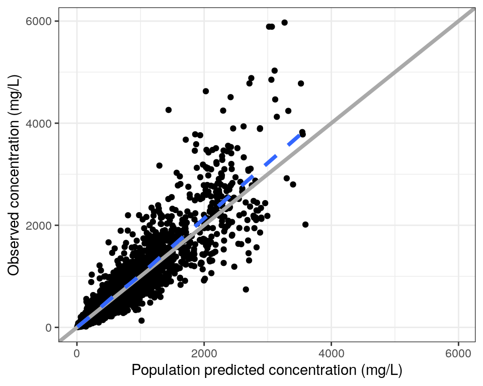

Figure 1: Observations versus population predictions of drug concentration. Observed values are indicated by solid black circles. The line of identity (solid grey) is included as a reference (x=y). The dashed blue line represents a LOESS smooth through the data.

dvip <- dv_ipred(data, yname = "concentration (mg/L)")
dvip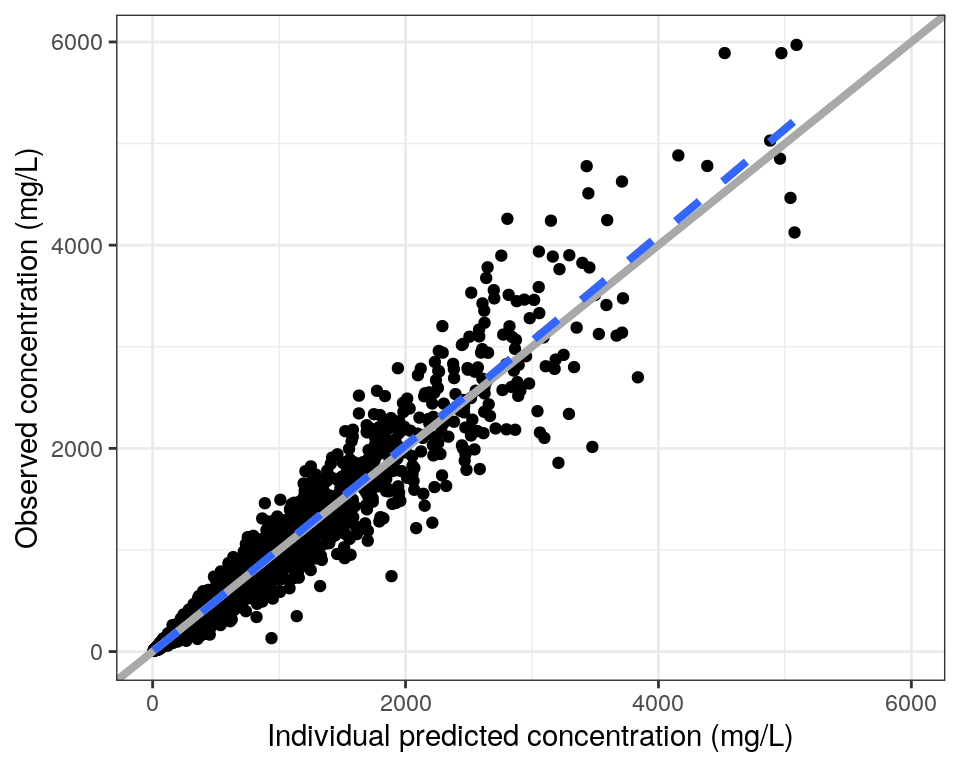

Figure 2: Observations versus individual predictions of drug concentration. Observed values are indicated by solid black circles. The line of identity (solid grey) is included as a reference (x=y). The dashed blue line represents a LOESS smooth through the data.

7.2 Individual observed vs predicted plots

Individual plots of DV, PRED and IPRED vs time (linear and log scale) are generated with the dv_pred_ipred function. These plots are highly customizable but here we show the first plot from a simple example

dvip <- dv_pred_ipred(
  data,
  id_per_plot = 9,
  ncol = 3,
  angle = 45,
  use_theme = theme_bw()
)
dvip[1]

$`1`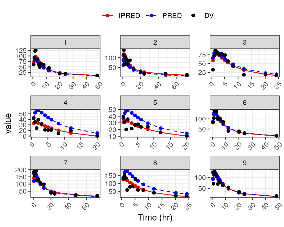

Figure 3: Observed (DV), population predicted (PRED) and individual predicted (IPRED) concentration versus time profiles, stratified by individual (ID).

7.3 NPDE Plots

The pmplots package includes a series of functions for plotting normalized prediction distribution errors (NPDEs):

npde_pred NPDE vs the population predictions (PRED)
npde_time NPDE vs time
npde_tad NPDE vs time after dose (TAD)
npde_cont NPDE vs continuous covariates
npde_cat NPDE vs categorical ocvariates
npde_hist distribution of NPDEs

Again, these functions can be customized and below we show how you can customize the axis labels using information in your spec file, how to map across multiple covariates and how to panel multiple plots into a single figure with the patchwork package.

7.3.1 NPDE vs population predictions, time and time after dose

The pmplots package provides basic, intuitive axes labels automatically for plots created using it’s functions. However, it also include a series of functions that you can use to customize those labels. Here we demonstrate how to grab the units for time from your spec object and append them to the time labels, and how to include your models specific endpoint with units (in this case, concentration (mg/L)).

xTIME <- pm_axis_time(spec$TIME$unit)
xTIME

[1] "TIME//Time (h)"

xTAD  <- pm_axis_tad(spec$TAD$unit)
xPRED <- glue(pm_axis_pred(), xname = "concentration (mg/L)")

p1 <- npde_pred(data, x = xPRED, y = "NPDE //  ")
p2 <- npde_time(data, x = xTIME)
p3 <- npde_tad(data, x = xTAD, y = "NPDE //  ")
p <- p1 / p2 / p3
p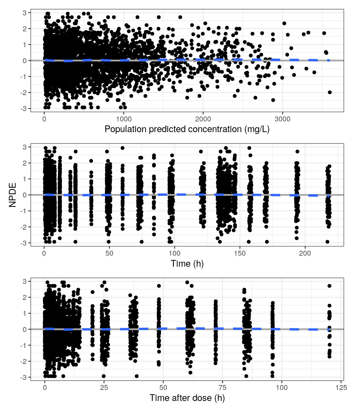

Figure 4: Normalized prediction distribution errors (NPDE) versus population predictions, time and time after dose. Solid black circles represent the individual residual values associated with each observation record. The solid horizontal grey line (residuals = 0) was included for reference. The dashed blue line represents a LOESS smooth through the data.

7.3.2 NPDE vs continuous covariates

The NPDE vs continuous covariate plots leverage the information in your spec object in two main ways:

the covariates of interest are extracted from the covariate flags in your spec file using the pull_meta function from yspec (also described above).
the axis labels are renamed with the short label in the spec

diagContCov <- pull_meta(spec, "flags")$diagContCov

NPDEco <- 
  spec %>% 
  ys_select(all_of(diagContCov)) %>%     
  axis_col_labs(title_case = TRUE, short_max = 10) %>%  
  as.list()

NPDEco

$AGE
[1] "AGE//Age (years)"

$WT
[1] "WT//Weight (kg)"

$ALB
[1] "ALB//Albumin (g/dL)"

$EGFR
[1] "EGFR//EGFR (mL/min/1.73m2)"

pList <- purrr::map(NPDEco, ~ npde_cont(data, x = .x))

pm_grid(pList, ncol = 2)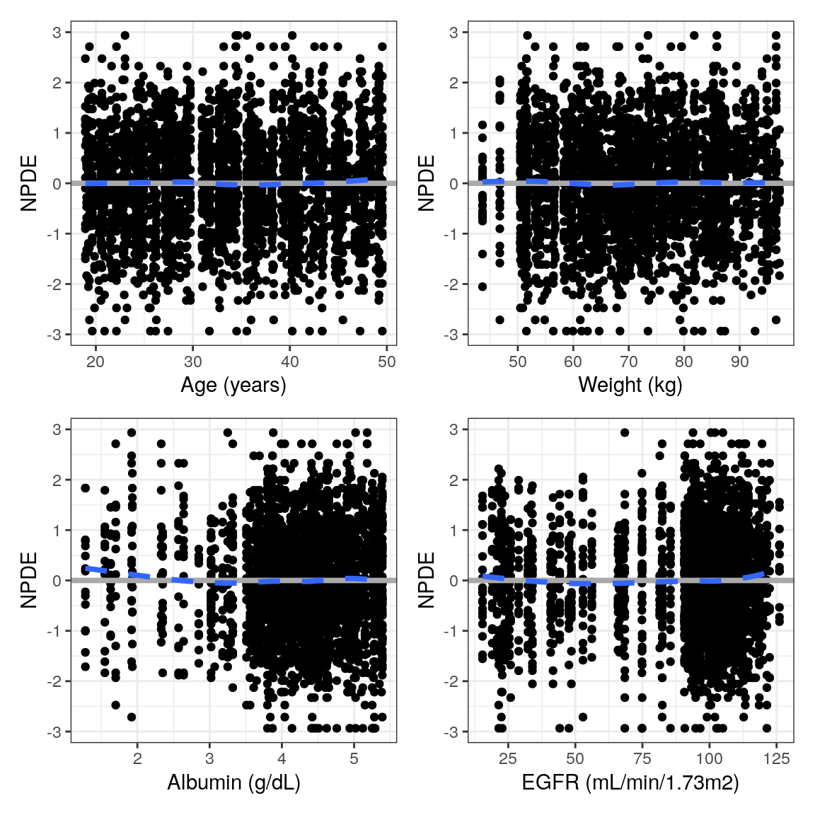

Figure 5: Normalized prediction distribution errors (NPDE) versus baseline continuous covariates. Solid black circles represent the individual NPDE values associated with each observation record. The solid horizontal grey line (residuals = 0) is included for reference. The dashed blue line represents a LOESS smooth through the data.

7.3.3 NPDE vs categorical covariates

As above, the information in the spec object was used to to rename the axis labels. These plots also used the spec object to decode the numerical categorical covariate categories (shown above).

NPDEca <- 
  spec %>% 
  ys_select("RF", "CP") %>% 
  axis_col_labs(title_case = TRUE, short_max = 20) %>%  
  as.list()
pList_cat = purrr::map(NPDEca, ~ npde_cat(data, x = .x))
pm_grid(pList_cat, ncol=1)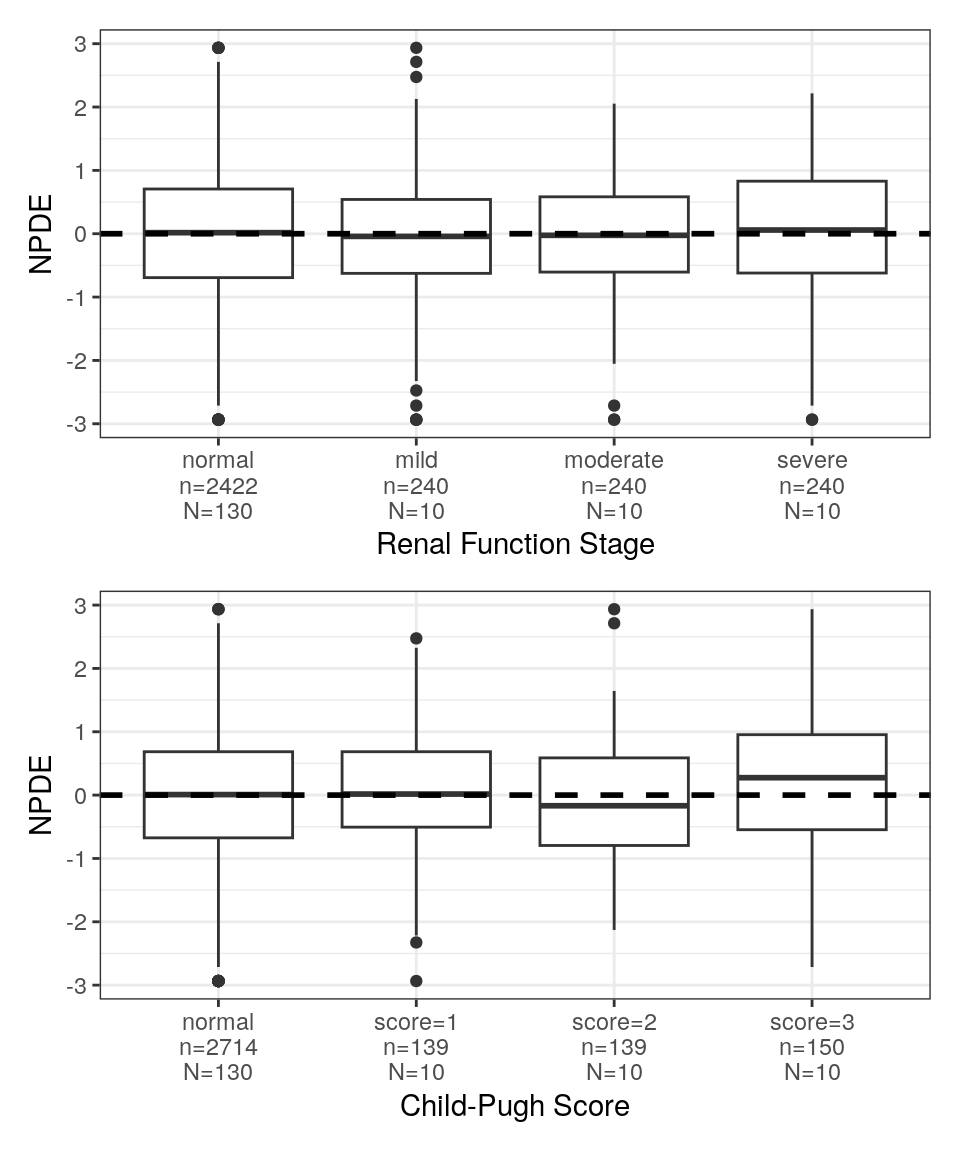

Figure 6: Normalized prediction distribution errors (NPDE) versus categorical covariates; renal function and child-pugh score. Median values are designated by a solid line in the center of the box. Boxes indicate the inter-quartile range (IQR) with whiskers extending to 1.5*IQR. A dashed black line at y = 0 is included as a reference. N = number of subjects, n = number of records.

7.3.4 NPDE histogram

Here we show an NPDE density plot but the y-axis can be customized to show count or density.

p <- npde_hist(data)
p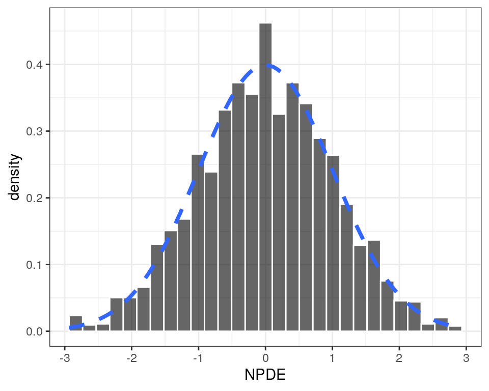

Figure 7: Normalized prediction distribution errors (NPDE) density plot.

7.4 Other residual plots

The pmplots package includes a similar series of functions to create other residual plots. They’re all similarly named but instead of beginning with npde_ they’re prefaced with

res_ for residual functions/plots
wres_ for weighted residual functions/plots
cwres_ for conditional weighted residual functions/plots
cwresi_ for conditional weighted residual with interaction functions/plots

Below are a couple of examples of CWRES plots.

7.4.1 CWRES vs population predictions, time and time after dose

p1 <- cwres_pred(data, x = xPRED, y = "CWRES //  ") 
p2 <- cwres_time(data, x = xTIME) 
p3 <- cwres_tad(data, x = xTAD, y = "CWRES //  ")
p <- p1 / p2 / p3
p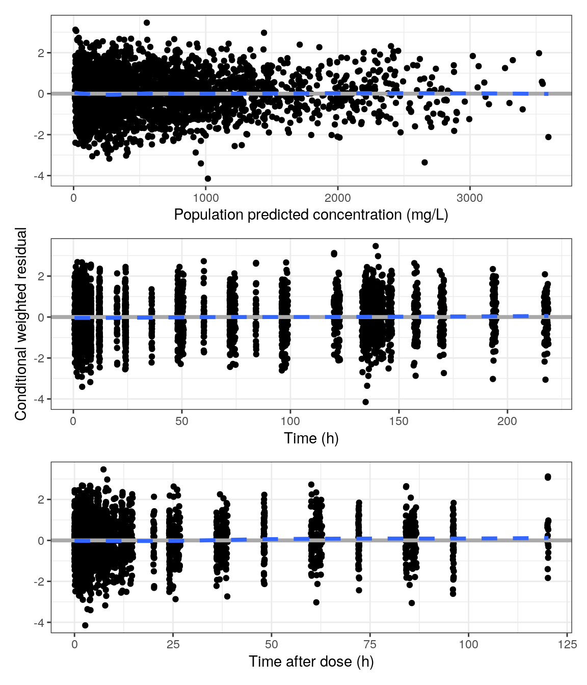

Figure 8: Conditional weighted residual (CWRES) versus population predictions and visit time. Solid black circles represent the individual CWRES values associated with each observation record. The solid horizontal grey line (residuals = 0) was included for reference. The dashed blue line represents a LOESS smooth through the data.

7.4.2 CWRES quantile-quantile (QQ) and density histogram

p <- cwres_q(data) / cwres_hist(data)
p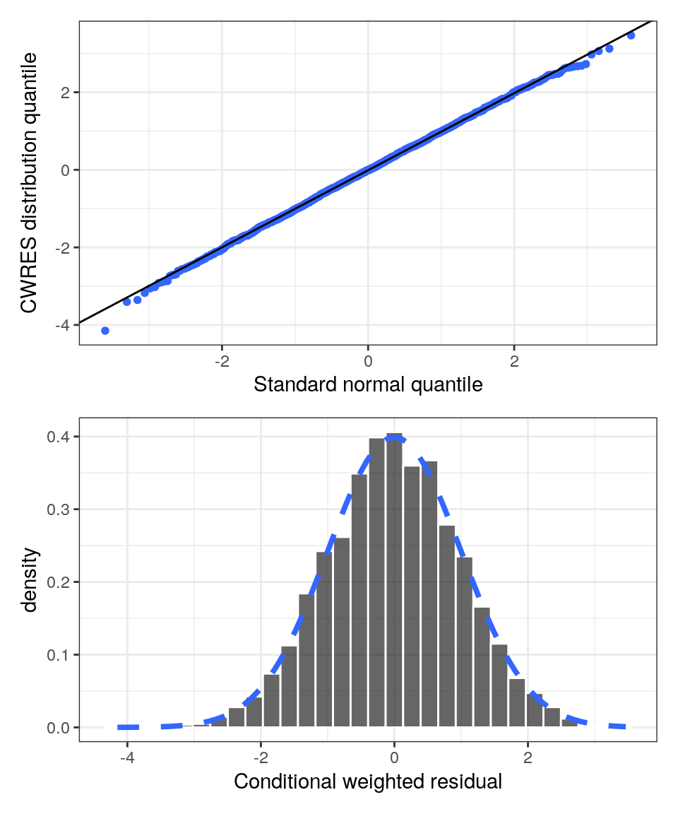

Figure 9: Conditional weighted residual (CWRES) quantile-quantile and density histogram. Quantile-quantile (Q-Q) plot - solid blue circles represent the CWRES values associated with each observation record. The solid black line (y=x) is included for reference. Density plot - density frequency (count) of the CWRES.

8 EBE-based diagnostics

The ETA based plots require a dataset filtered to one record per subject

id <- distinct(data, ID, .keep_all=TRUE)

Here we show how to plot:

eta_pairs the correlation and distribution of model ETAs
eta_cont ETA vs continous covariates
eta_cat ETA vs categorical covariates

Again we’ll leverage the information in the spec object in several ways:

the covariates of interest are extracted from the covariate flags in your spec file using the pull_meta function and those covariates are selected from the spec object using ys_select function (also described above).
the axis labels are renamed with the short label in the spec using axis_col_labs
numerical categorical covariates are decoded with the yspec_add_factors function

The ETAs to be plotted can either be extracted programatically

etas <- stringr::str_subset(names(data), "ETA")

or you can create a list with labels that replace the ETA numbers in your plots

etas <- c("ETA1//ETA-KA", "ETA2//ETA-V/F", "ETA3//ETA-CL/F")

8.1 ETA pairs plot

p <- eta_pairs(id, etas)
p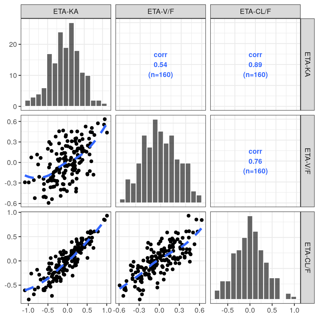

Figure 10: Correlation and distribution of individual estimates of interindividual and interoccasion variability. The lower off-diagonal shows a bivariate scatter plot with values indicated by black circles and a dashed blue LOESS smooth trend line through the data. The diagonal shows density frequency (count) plots of the data, and the correlation coefficient is reported in the upper off-diagonal.

8.2 ETA vs continuous covariates

Here we use a map_wrap_eta_cont function to generate plots of all continuous covariates vs each ETA value in a single line. Note that in this case we map over the ETAs and produce one plot per ETA faceted by continous covariates. Below we show a similar example for categorical covariates but there we’ll create one plot per covariate and ETA pair. For brevity we’ll show an example of the first plot but the code produces one plot per ETA.

map_wrap_eta_cont function code

##' Purpose: plot ETA vs all continuous covariates
##' @param  .map_etas character: name of ETA
##' @param  .co       string: continuous covariate list
##' @param  .id       dataframe: includes one record per id
##' @param  .ncol     number of columns in the plot
map_wrap_eta_cont <- function(.map_etas,.co,.id, .ncol=2) {
  .p <- wrap_eta_cont(
    .id,
    y = .map_etas,
    x = .co,
    use_labels = TRUE,
    ncol = .ncol, scales= "free_x"
  )
}

co <- 
  spec %>% 
  ys_select(all_of(diagContCov)) %>%    
  axis_col_labs(title_case = TRUE, short_max = 10)

p <- purrr::map(.x = etas, ~ map_wrap_eta_cont(.x, co, id))
p[[1]]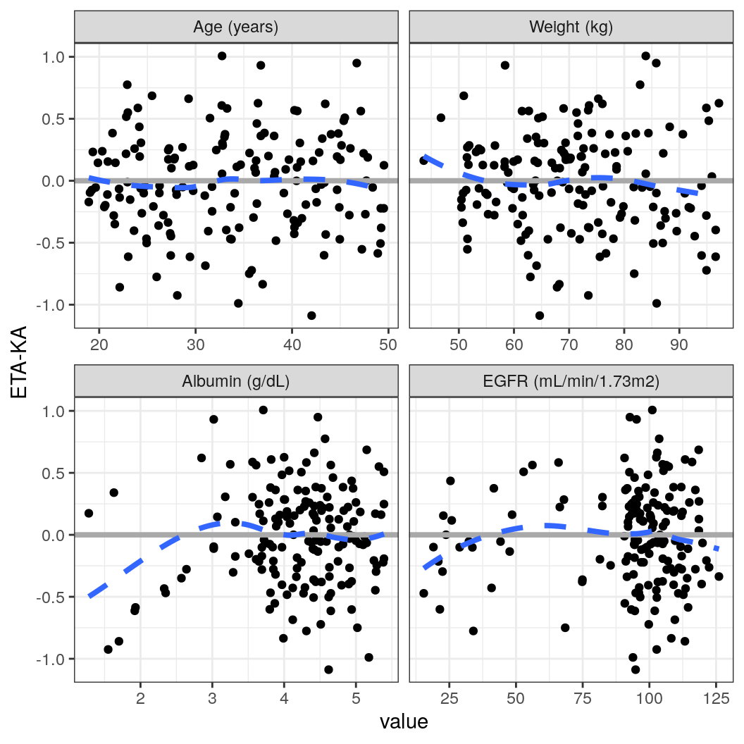

Figure 11: Individual estimates of interindividual variability (IIV) on the absorption rate constant (KA) versus baseline continuous covariates. Black points represent data points with the blue dashed line representing a LOESS smooth through the data. The solid horizontal grey line (residual = 0) is included for reference.

8.3 ETA vs categorical covariate

Here we show how to map over the categorical covariates of interest and to create one plot per covariate and ETA pair. These plots can be combined using the patchwork package.

ca <- 
  spec %>% 
  ys_select(diagCatCov) %>% 
  axis_col_labs(title_case=TRUE, short_max = 20)

Warning: Using an external vector in selections was deprecated in tidyselect 1.1.0.
ℹ Please use `all_of()` or `any_of()` instead.
  # Was:
  data %>% select(diagCatCov)

  # Now:
  data %>% select(all_of(diagCatCov))

See <https://tidyselect.r-lib.org/reference/faq-external-vector.html>.

p <- eta_cat(id, ca, etas)
pRenal <- (p[[5]] + p[[6]]) / (p[[7]] + p[[8]])
pRenal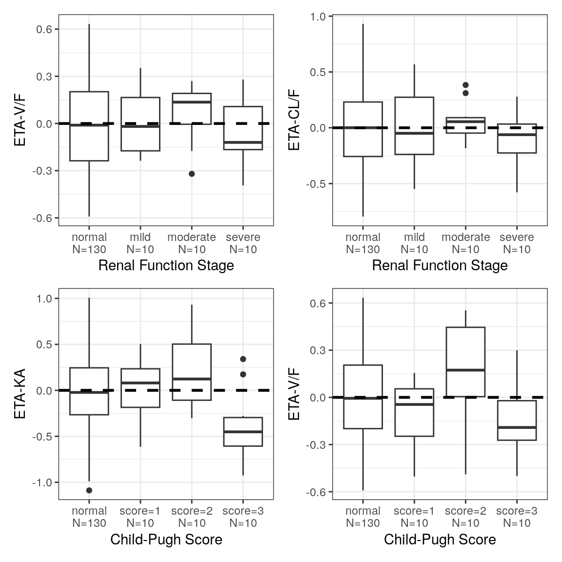

Figure 12: Individual estimates of interindividual variability (IIV) versus renal function. Median values are designated by a solid line in the center of the box. Boxes indicate the inter-quartile range (IQR) with whiskers extending to 1.5*IQR. A dashed black line at y = 0 is included as a reference. N = number of subjects.

9 Other resources

The scripts discussed on this page can be found in the Github repository. To run this code you should consider visiting the About the Github Repo page first.

9.1 Diagnostic templates

Code shown on this page is available: diagnostics-report.Rmd.
The code to create individual observed vs predicted plots (DV, PRED and IPRED vs time, linear and log scale) is available: id-dv-pred-plots.Rmd.

9.2 Diagnostic scripts

The functions (not in packages) used in these diagnostics is available here: functions-diagnostics.R.
The code to render these model diagnostics as a parameterized report is available: model-diagnostics.R.

9.3 Publications

Nguyen et al. Model Evaluation of Continuous Data Pharmacometric Models: Metrics and Graphics. CPT Pharmacometrics Syst Pharmacol. 2017 Feb;6(2):87-109.
Byon et al. Establishing best practices and guidance in population modeling: an experience with an internal population pharmacokinetic analysis guidance. CPT Pharmacometrics Syst Pharmacol. 2013 Jul 3;2(7):e51. doi: 10.1038/psp.2013.26. PMID: 23836283; PMCID: PMC6483270.