library(bbr)
library(pmtables)
library(dplyr)
library(here)

source(here("script", "functions-model.R"))

MODEL_DIR <- here("model", "pk")
FIGURE_DIR <- here("deliv", "figure")1 Introduction
Our model summaries provide a condensed overview of the key decisions made during the model development process. They’re quick to compile and take advantage of the easy annotation features of bbr, such as the description, notes, and tags, to summarize the important features of key models.
The page demonstrates how to:
- Create and modify model run logs
- Check and compare model tags
- Pull in key diagnostics to support modeling decisions
For a walk-though on how to define, submit and annotate your models, see the Model Management. Guidance for creating model diagnostics are given on the Model Diagnostics and Parameterized Reports for Model Diagnostics pages.
2 Tools used
2.1 MetrumRG packages
bbr Manage, track, and report modeling activities, through simple R objects, with a user-friendly interface between R and NONMEM®.
pmtables Create summary tables commonly used in pharmacometrics and turn any R table into a highly customized tex table.
2.2 CRAN packages
dplyr A grammar of data manipulation.
knitr General-purpose literate programming engine.
3 Outline
During model development you often make a series of decisions regarding which models to test and which direction to take. Here we demonstrate how you can use a series of bbr functions, and the model annotation, to summarize these key choices and decisions. We recommend creating this model summary in an RMarkdown that can be knit throughout the project to quickly compile a well formatted summary document you can share with other project collaborators, group leaders, etc.
4 Set up
Load required packages, any helper functions and set the file path to your model directory.
5 Create a run log
A run log table summarizing the important models is often included in a final report when the analysis is complete. However, it can also be useful along the way as a tool for reviewing the models you’ve already tried and determining what you may want to try next.
The ?run_log function reads in the annotation attached to your models (in Model Management) and some metadata that bbr tracks for you. By default, it finds all models in the directory that you pass it and can optionally search recursively in sub-directories.
log_df <- run_log(MODEL_DIR)
names(log_df)
[1] "absolute_model_path" "run" "yaml_md5"
[4] "model_type" "description" "bbi_args"
[7] "based_on" "tags" "notes"
[10] "star" You can explore this tibble with View(log_df) in Rstudio or you could use dplyr to select the columns to display, and then knitr::kable() to create a well formatted HTML table to include in your knit document.
log_df %>%
  select(run, based_on, description, tags, notes) %>%
collapse_to_string(tags, notes) %>% knitr::kable()| run | based_on | description | tags | notes |
|---|---|---|---|---|
| 100 | NULL | NA | one-compartment + absorption, ETA-CL, ETA-KA, ETA-V, proportional RUV | systematic bias, explore alternate compartmental structure |
| 101 | 100 | NA | two-compartment + absorption, ETA-CL, ETA-KA, ETA-V2, proportional RUV | eta-V2 shows correlation with weight, consider adding allometric weight |
| 102 | 101 | Base Model | two-compartment + absorption, ETA-CL, ETA-KA, ETA-V2, CLWT-allo, V2WT-allo, QWT-allo, V3WT-allo, proportional RUV | Allometric scaling with weight reduces eta-V2 correlation with weight. Will consider additional RUV structures, Proportional RUV performed best over additive (103) and combined (104) |
| 103 | 102 | NA | two-compartment + absorption, ETA-CL, ETA-KA, ETA-V2, CLWT-allo, V2WT-allo, QWT-allo, V3WT-allo, additive RUV | Additive only RUV performs poorly and will not consider going forward. |
| 104 | 102 | NA | two-compartment + absorption, ETA-CL, ETA-KA, ETA-V2, CLWT-allo, V2WT-allo, QWT-allo, V3WT-allo, combined RUV | Combined RUV performs only slightly better than proportional only, should look at parameter estimates for 104, CI for Additive error parameter contains zero and will not be used going forward |
| 105 | 102 | NA | two-compartment + absorption, ETA-CL, ETA-KA, ETA-V2, CLWT-allo, V2WT-allo, QWT-allo, V3WT-allo, CLEGFR, CLAGE, proportional RUV | Pre-specified covariate model |
| 106 | 105 | Final Model | two-compartment + absorption, ETA-CL, ETA-KA, ETA-V2, CLWT-allo, V2WT-allo, QWT-allo, V3WT-allo, CLEGFR, CLAGE, CLALB, proportional RUV | Client was interested in adding Albumin to CL |
| 999 | 106 | NA | NA | Simulation run |
The ?collapse_to_string function is a simple formatting helper to combine the vector of notes or tags into a single string for better display.
6 Check your model and data files
bbr records the state of your control stream and input data at the time the model was run. This allows you to easily check if either the model or data file has changed since the model was run. This is useful for catching models that may need to be re-run.
The bbr::check_up_to_date() function is described in more detail in the Checking if models are up-to-date section of the “Getting Started” vignette. Here we use it for its side effect of printing a warning if any model or data files in the run log models have changed.
# check if model or data files have changed (from bbr)
check_up_to_date(log_df)
7 Add diagnostics to your run log
The bbr::summary_log() function extracts some basic diagnostics from a batch of models by running ?summary_log (discussed in more detail in Model Management) on each model. It finds and extracts elements of those model summaries into a tibble with one model per row. This function is discussed in more detail in the Creating summary log vignette).
These diagnostic columns can be appended to your run log using add_summary() as follows:
log_df <- add_summary(log_df)
log_df %>%
select(run, ofv, param_count, any_heuristics) %>% knitr::kable()| run | ofv | param_count | any_heuristics |
|---|---|---|---|
| 100 | 33502.96 | 10 | TRUE |
| 101 | 31185.58 | 12 | FALSE |
| 102 | 30997.91 | 12 | FALSE |
| 103 | 36411.27 | 12 | FALSE |
| 104 | 30997.71 | 13 | FALSE |
| 105 | 30928.82 | 14 | FALSE |
| 106 | 30904.41 | 15 | FALSE |
| 999 | NA | NA | NA |
Using bbr::add_summary() adds roughly 20 columns to your log_df tibble (details on all the columns can be found in ?summary_log). Here we select only the objective function value (ofv), count of non-fixed parameters (param_count), and the boolean flag indicating if any heuristics were triggered (any_heuristics).
9 Creating a report-ready run log table
While a run log can be useful for checking the state of a project, they’re also often included in the final report. MetrumRGs reports are written in Latex and report-ready run log tables are created by passing the run log tibble to the pmtables package:
log_df %>%
  select(run, based_on, description, tags) %>%
  collapse_to_string(tags) %>%
  st_new() %>%
  st_left(tags = col_ragged(8)) %>% # fix column width for text-wrapping
  st_as_image()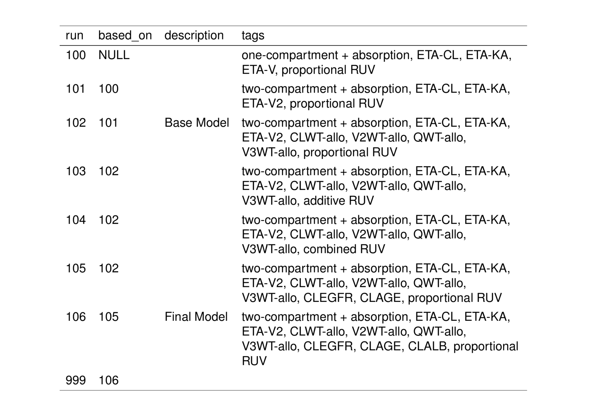
10 Modeling notes
Depending on the project, it can be helpful to include some detail on important models or key decisions made during model development to complement the run log.
While the intent is capture notes, plots or tables for select models, there are only seven models in this Expo and so you’ll see them all represented here. In a real project, only models that would help others (or your future self) follow your logic at key decision points would be included.
Below are some examples using bbr and dplyr, along with the figures we generated with Parameterized Reports for Model Diagnostics, to highlight decision points in the Expo model development.
10.1 Model 100-101: Compartments
Compare the objective function value for models 100 (one compartment) and 101 (two compartment):
compare_ofv(100:101, log_df)| run | ofv | tags |
|---|---|---|
| 100 | 33502.96 | one-compartment + absorption, ETA-CL, ETA-KA, ETA-V, proportional RUV |
| 101 | 31185.58 | two-compartment + absorption, ETA-CL, ETA-KA, ETA-V2, proportional RUV |
The compare_ofv function (in functions-model.R) filters the summary log tibble to only the specified columns.
Compare CWRES between models 100 and 101.
knitr::include_graphics(file.path(FIGURE_DIR, "100/100-cwres-pred-time-tad.pdf"))knitr::include_graphics(file.path(FIGURE_DIR, "101/101-cwres-pred-time-tad.pdf"))Second compartment reduces the objective function and residual issues.
10.2 Model 101-102: Covariates
Look at the ETAs versus covariates plots to assess potential covariate effects.
mod101 <- read_model(file.path(MODEL_DIR, 101))
print(mod101$notes)
[1] "eta-V2 shows correlation with weight, consider adding allometric weight"knitr::include_graphics(file.path(FIGURE_DIR, "101/101-eta-all-cont-cov.pdf"))knitr::include_graphics(file.path(FIGURE_DIR, "102/102-eta-all-cont-cov.pdf"))10.3 Models 102-104: Error structure
Compare proportional, additive, or combined error models for the residual unexplained variability (RUV).
compare_ofv(102:104, log_df, notes)| run | ofv | tags | notes |
|---|---|---|---|
| 102 | 30997.91 | two-compartment + absorption, ETA-CL, ETA-KA, ETA-V2, CLWT-allo, V2WT-allo, QWT-allo, V3WT-allo, proportional RUV | Allometric scaling with weight reduces eta-V2 correlation with weight. Will consider additional RUV structures, Proportional RUV performed best over additive (103) and combined (104) |
| 103 | 36411.27 | two-compartment + absorption, ETA-CL, ETA-KA, ETA-V2, CLWT-allo, V2WT-allo, QWT-allo, V3WT-allo, additive RUV | Additive only RUV performs poorly and will not consider going forward. |
| 104 | 30997.71 | two-compartment + absorption, ETA-CL, ETA-KA, ETA-V2, CLWT-allo, V2WT-allo, QWT-allo, V3WT-allo, combined RUV | Combined RUV performs only slightly better than proportional only, should look at parameter estimates for 104, CI for Additive error parameter contains zero and will not be used going forward |
10.4 Models 105-106: Final model candidates
Model 105 adds pre-specified covariates while model 106 includes an additional effect of albumin on CL/F (requested by a collaborator).
Filter the run logs to only models with relevant covariate tags:
run_log(MODEL_DIR, .include = TAGS$cov_cl_egfr) %>%
  add_summary() %>%
  select(run, tags, ofv, param_count, condition_number) %>%
collapse_to_string(tags) %>% knitr::kable()| run | tags | ofv | param_count | condition_number |
|---|---|---|---|---|
| 105 | two-compartment + absorption, ETA-CL, ETA-KA, ETA-V2, CLWT-allo, V2WT-allo, QWT-allo, V3WT-allo, CLEGFR, CLAGE, proportional RUV | 30928.82 | 14 | 53.8711 |
| 106 | two-compartment + absorption, ETA-CL, ETA-KA, ETA-V2, CLWT-allo, V2WT-allo, QWT-allo, V3WT-allo, CLEGFR, CLAGE, CLALB, proportional RUV | 30904.41 | 15 | 48.5125 |
10.5 Comparing base and final models
log_df %>%
  filter(star) %>%
  select(run, description, tags, ofv, param_count) %>%
collapse_to_string(tags) %>% knitr::kable()| run | description | tags | ofv | param_count |
|---|---|---|---|---|
| 102 | Base Model | two-compartment + absorption, ETA-CL, ETA-KA, ETA-V2, CLWT-allo, V2WT-allo, QWT-allo, V3WT-allo, proportional RUV | 30997.91 | 12 |
| 106 | Final Model | two-compartment + absorption, ETA-CL, ETA-KA, ETA-V2, CLWT-allo, V2WT-allo, QWT-allo, V3WT-allo, CLEGFR, CLAGE, CLALB, proportional RUV | 30904.41 | 15 |
mod102 <- read_model(file.path(MODEL_DIR, 102))
mod106 <- read_model(file.path(MODEL_DIR, 106))

tags_diff(mod102, mod106)
In 102 but not 106:
In 106 but not 102: CLEGFR, CLAGE, CLALBmodel_diff(mod102, mod106)@@ 1,3 @@@@ 1,3 @@<$PROBLEM From bbr: see 102.yaml for details>$PROBLEM From bbr: see 106.yaml for details$INPUT C NUM ID TIME SEQ CMT EVID AMT DV AGE WT HT EGFR ALB BMI SEX AAG$INPUT C NUM ID TIME SEQ CMT EVID AMT DV AGE WT HT EGFR ALB BMI SEX AAG@@ 14,10 @@@@ 14,14 @@V2WT = LOG(WT/70)V2WT = LOG(WT/70)CLWT = LOG(WT/70)*0.75CLWT = LOG(WT/70)*0.75~>CLEGFR = LOG(EGFR/90)*THETA(6)~>CLAGE = LOG(AGE/35)*THETA(7)V3WT = LOG(WT/70)V3WT = LOG(WT/70)QWT = LOG(WT/70)*0.75QWT = LOG(WT/70)*0.75~>CLALB = LOG(ALB/4.5)*THETA(8)~>KA = EXP(THETA(1)+ETA(1))KA = EXP(THETA(1)+ETA(1))V2 = EXP(THETA(2)+V2WT+ETA(2))V2 = EXP(THETA(2)+V2WT+ETA(2))<CL = EXP(THETA(3)+CLWT+ETA(3))>CL = EXP(THETA(3)+CLWT+CLEGFR+CLAGE+CLALB+ETA(3))V3 = EXP(THETA(4)+V3WT)V3 = EXP(THETA(4)+V3WT)Q = EXP(THETA(5)+QWT)Q = EXP(THETA(5)+QWT)@@ 35,5 @@@@ 39,7 @@(4) ; 4 V3 (L) - 70(4) ; 4 V3 (L) - 70(2) ; 5 Q (L/hr) - 4(2) ; 5 Q (L/hr) - 4<>(1) ; 6 CLEGFR~CL ()~>(1) ; 7 AGE~CL ()~>(0.5) ; 8 ALB~CL ()$OMEGA BLOCK(3)$OMEGA BLOCK(3)@@ 45,6 @@@@ 51,5 @@0.05 ; 1 pro error0.05 ; 1 pro error<$EST MAXEVAL=9999 METHOD=1 INTER SIGL=6 NSIG=3 PRINT=1 RANMETHOD=P MSFO=./102.msf>$EST MAXEVAL=9999 METHOD=1 INTER SIGL=6 NSIG=3 PRINT=1 RANMETHOD=P MSFO=./106.msf$COV PRINT=E RANMETHOD=P$COV PRINT=E RANMETHOD=P<$TABLE NUM IPRED NPDE CWRES NOPRINT ONEHEADER RANMETHOD=P FILE=102.tab>$TABLE NUM IPRED NPDE CWRES CL V2 Q V3 KA ETAS(1:LAST) NOPRINT ONEHEADER RANMETHOD=P FILE=106.tab<$TABLE NUM CL V2 Q V3 KA ETAS(1:LAST) NOAPPEND NOPRINT ONEHEADER FILE=102par.tab~
10.6 Summarize final model
mod106 %>%
  model_summary() %>%
  param_estimates() %>%
mutate(across(where(is.numeric), pmtables::sig)) %>% knitr::kable()| parameter_names | estimate | stderr | random_effect_sd | random_effect_sdse | fixed | diag | shrinkage |
|---|---|---|---|---|---|---|---|
| THETA1 | 0.443 | 0.0643 | NA | NA | FALSE | NA | NA |
| THETA2 | 4.12 | 0.0275 | NA | NA | FALSE | NA | NA |
| THETA3 | 1.17 | 0.0280 | NA | NA | FALSE | NA | NA |
| THETA4 | 4.21 | 0.0190 | NA | NA | FALSE | NA | NA |
| THETA5 | 1.28 | 0.0348 | NA | NA | FALSE | NA | NA |
| THETA6 | 0.485 | 0.0395 | NA | NA | FALSE | NA | NA |
| THETA7 | -0.0378 | 0.0635 | NA | NA | FALSE | NA | NA |
| THETA8 | 0.419 | 0.0863 | NA | NA | FALSE | NA | NA |
| OMEGA(1,1) | 0.219 | 0.0526 | 0.468 | 0.0562 | FALSE | TRUE | 14.4 |
| OMEGA(2,1) | 0.0668 | 0.0194 | 0.498 | 0.0997 | FALSE | FALSE | NA |
| OMEGA(2,2) | 0.0824 | 0.00981 | 0.287 | 0.0171 | FALSE | TRUE | 5.51 |
| OMEGA(3,1) | 0.121 | 0.0224 | 0.767 | 0.0823 | FALSE | FALSE | NA |
| OMEGA(3,2) | 0.0704 | 0.00918 | 0.725 | 0.0418 | FALSE | FALSE | NA |
| OMEGA(3,3) | 0.114 | 0.0128 | 0.338 | 0.0189 | FALSE | TRUE | 1.25 |
| SIGMA(1,1) | 0.0399 | 0.00123 | 0.200 | 0.00309 | FALSE | TRUE | 5.02 |
11 Other resources
The following script from the Github repository is discussed on this page. If you’re interested running this code, visit the About the Github Repo page first.
- Model summary script:
model-summary.Rmd