Introduction

Managing model development processes in a traceable and reproducible manner can be a significant challenge. At Metrum Research Group (MetrumRG), we use bbr and bbr.bayes to streamline this process for fitting Bayesian (Bayes) models using NONMEM®. bbr and bbr.bayes are R packages developed by MetrumRG that serve three primary purposes:

Submit NONMEM® models, particularly for execution in parallel and/or on a high-performance compute (HPC) cluster (e.g. Metworx).
Parse NONMEM® outputs into R objects to facilitate model evaluation and diagnostics in R.
Annotate the model development process for easier and more reliable traceability and reproducibility.

This page demonstrates the following bbr and bbr.bayes functionality:

Create a Bayes NONMEM® model either from scratch or based on a model previously developed using another estimation method such as FOCE
Submit a model
Markov Chain Monte Carlo (MCMC) diagnostics
Model diagnostics
Iterative model development
Annotation of models with tags, notes, etc.,

Tools used

MetrumRG packages

bbr Manage, track, and report modeling activities, through simple R objects, with a user-friendly interface between R and NONMEM®.

bbr.bayes Extension of the bbr package to support Bayesian modeling with Stan or NONMEM®.

CRAN packages

dplyr A grammar of data manipulation.

Outline

This page details a range of tasks typically performed throughout the modeling process such as defining, submitting, and annotating models. Our scientists run this code in a scratch pad style script (i.e., model-management.R) because it isn’t necessary for the entire coding history for each model to persist. Here, the code used each step of the process is provided as a reference, and a runnable version of this page is available in our Github repository: model-management-demo.Rmd.

If you’re a new bbr user, we recommend you read through the Getting Started vignette before trying to run any code. This vignette includes some setup and configuration (e.g., making sure bbr can find your NONMEM® installation) that needs to be done.

Please note that bbr doesn’t edit the model structure in your control stream. This page walks through a sequence of models that might evolve during a Bayes modeling project. All modifications to the control streams were made directly by the user in the control stream. Below we include comments asking you to edit your control streams manually.

Set up

Load required packages and set file paths to your model and figure directories.

library(bbr)
library(bbr.bayes)
library(dplyr)
library(here)

MODEL_DIR <- here("model", "pk")
MODEL_DIR_sim <- here("script", "model")
FIGURE_DIR <- here("deliv", "figure")

Model creation and submission

Previous FOCE model

This example picks up at the end of a completed, base-model development process. Assume we have a base model developed in another estimation method like FOCE. Here, we actually use model 102 from MeRGE Expo 1.

mod102 <- read_model(file.path(MODEL_DIR, 102))

Copy FOCE model to a Bayesian model object

This model is now copied to a new control stream, 1000.ctl, using the function bbr.bayes::copy_model_as_nmbayes(). We construct the bbr model object and replace one of the model tags after reading in the tags file. Model tags are described in more detail here.

The first argument to copy_model_as_nmbayes() is the model object read in above, and the second is a path to your new model control stream without the file extension.

TAGS <- yaml::read_yaml(here("script", "tags.yaml"))
mod1000 <- copy_model_as_nmbayes(
  mod102,
  file.path(MODEL_DIR, 1000),
  .inherit_tags = TRUE
) %>%
  replace_tag(TAGS$foce, TAGS$bayes)

Edit your control stream

The model structure is copied exactly from the FOCE model to the new Bayes model, but there are a couple of changes we need to make to the control stream:

Add priors
Define settings for the MCMC chains, including the number of chains, number of samples, and how initial values are generated

We walk through how to make these changes, but the specific settings for your model is out of scope of this Expo. For those topics, we refer readers to the following publication:

Johnston CK, Waterhouse T, Wiens M, Mondick J, French J, Gillespie WR. Bayesian estimation in NONMEM. CPT Pharmacometrics Syst Pharmacol. 2023; 00: 1-16. doi.org/10.1002/psp4.13088

You need to manually edit the new control stream with these modifications. If you’re using RStudio (or any other editor supported by utils::file.edit()), you can easily open your control stream for editing with the following:

mod1000 %>% open_model_file()

The following lines are automatically added to the control stream, replacing the previous $ESTIMATION block:

; TODO: This model was copied by bbr.bayes::copy_model_as_nmbayes().
;       nmbayes models require a METHOD=CHAIN estimation record and a
;       METHOD=BAYES or METHOD=NUTS estimation record. The records
;       below are meant as a starting point.  At the very least, you
;       need to adjust the number of iterations (see NITER option in
;       the second $EST block), but please review all options
;       carefully.
;
;       See ?bbr.bayes::bbr_nmbayes and the NONMEM docs for details.
$EST METHOD=CHAIN FILE={model_id}.chn NSAMPLE=4 ISAMPLE=0 SEED=1
     CTYPE=0 IACCEPT=0.3 DF=10 DFS=0

$EST METHOD=NUTS SEED=1 NBURN=250 NITER=NNNN
     AUTO=2 CTYPE=0 OLKJDF=2 OVARF=1
     NUTS_DELTA=0.95 PRINT=10 MSFO={model_id}.msf RANMETHOD=P PARAFPRINT=10000
     BAYES_PHI_STORE=1

For this example, we run four separate chains for each model. Each chain uses a different random seed and a different set of initial estimates. The file 1000.ctl is actually a template control stream that bbr.bayes uses to create the four separate model files. We make use of METHOD=CHAIN in NONMEM® to generate the initial estimates and, subsequently, read those values in when running each chain.

bbr.bayes requires that the control stream includes a line with

$EST METHOD=CHAIN FILE=xyz.chn NSAMPLE=4 ISAMPLE=0 ...

where xyz.chn is the file with initial estimates for model number xyz, and NSAMPLE is the number of chains. ISAMPLE is set accordingly when running each chain. But, this initial value of 0 is set to generate the initial estimates rather than read them in.

Also, bbr has several helper functions to help update your control stream. For example, the defined suffixes can be updated directly from your R console. The update_model_id function updates the defined suffixes from {parent_mod}.{suffix} to {current_mod}.{suffix} in your new control stream for the following file extensions:

.MSF
.EXT
.CHN
.tab
par.tab

mod1000 <- update_model_id(mod1000)

You can easily look at the differences between control streams of a model and its parent model. The main differences here include new MU referencing, additional prior distributions, and updated the estimation method.

model_diff(mod1000)

<
 
1000
>
 
102
@@ 1,3 @@
@@ 1,3 @@
<
 
$PROBLEM 1000
>
 
$PROBLEM From bbr: see 102.yaml for details
 
 
 
 
 
 
 
 
$INPUT C NUM ID TIME SEQ CMT EVID AMT DV AGE WT HT EGFR ALB BMI SEX AAG
 
 
$INPUT C NUM ID TIME SEQ CMT EVID AMT DV AGE WT HT EGFR ALB BMI SEX AAG
@@ 13,31 @@
@@ 13,21 @@
 
 
 
 
 
 
 
 
  V2WT   = LOG(WT/70)
 
 
V2WT = LOG(WT/70)
<
 
  CLWT   = LOG(WT/70) * 0.75
>
 
CLWT = LOG(WT/70)*0.75
 
 
  V3WT   = LOG(WT/70)
 
 
V3WT = LOG(WT/70)
<
 
  QWT    = LOG(WT/70) * 0.75
>
 
QWT  = LOG(WT/70)*0.75
<
 
 
~
 
<
 
  MU_1   = THETA(1)
~
 
<
 
  MU_2   = THETA(2) + V2WT
~
 
<
 
  MU_3   = THETA(3) + CLWT
~
 
<
 
  MU_4   = THETA(4) + V3WT
~
 
<
 
  MU_5   = THETA(5) + QWT
~
 
<
 
 
~
 
<
 
  ;" CALL EXTRASEND()
~
 
 
 
 
 
 
 
<
 
  KA     = EXP(MU_1 + ETA(1))
>
 
KA   = EXP(THETA(1)+ETA(1))
<
 
  V2     = EXP(MU_2 + ETA(2))
>
 
V2   = EXP(THETA(2)+V2WT+ETA(2))
<
 
  CL     = EXP(MU_3 + ETA(3))
>
 
CL   = EXP(THETA(3)+CLWT+ETA(3))
<
 
  V3     = EXP(MU_4 + ETA(4))
>
 
V3   = EXP(THETA(4)+V3WT)
<
 
  Q      = EXP(MU_5 + ETA(5))
>
 
Q    = EXP(THETA(5)+QWT) 
 
 
 
 
 
 
 
 
  S2     = V2/1000 ; dose in mcg, conc in mcg/mL
 
 
S2 = V2/1000 ; dose in mcg, conc in mcg/mL
 
 
 
 
 
 
 
 
$ERROR
 
 
$ERROR
<
 
 
~
 
 
 
  IPRED = F
 
 
IPRED = F 
<
 
  Y     = IPRED * (1 + EPS(1))
>
 
Y=IPRED*(1+EPS(1))
 
 
 
 
 
 
<
 
$THETA
>
 
$THETA  ; log values
<
 
; log values
~
 
 
 
  (0.5)         ; 1 KA (1/hr) - 1.5
 
 
(0.5)   ;  1 KA (1/hr) - 1.5
 
 
  (3.5)         ; 2 V2 (L) - 60
 
 
(3.5)   ;  2 V2 (L) - 60
@@ 45,37 @@
@@ 35,16 @@
 
 
  (4)           ; 4 V3 (L) - 70
 
 
(4)     ;  4 V3 (L) - 70
 
 
  (2)           ; 5 Q  (L/hr) - 4
 
 
(2)     ;  5 Q  (L/hr) - 4
~
 
>
 
 
 
 
 
 
 
 
 
 
$OMEGA BLOCK(3)
 
 
$OMEGA BLOCK(3)
<
 
  0.2           ; ETA(KA)
>
 
0.2   ;ETA(KA)
<
 
  0.01 0.2      ; ETA(V2)
>
 
0.01 0.2   ;ETA(V2)
<
 
  0.01 0.01 0.2 ; ETA(CL)
>
 
0.01 0.01 0.2   ;ETA(CL)
<
 
$OMEGA
~
 
<
 
  0.025 FIX    ; ETA(V3)
~
 
<
 
  0.025 FIX    ; ETA(Q)
~
 
 
 
 
 
 
 
 
 
$SIGMA
 
 
$SIGMA
 
 
  0.05          ; 1 pro error
 
 
0.05     ; 1 pro error
<
 
 
~
 
<
 
$PRIOR NWPRI
~
 
 
 
 
 
 
 
<
 
$THETAP
>
 
$EST MAXEVAL=9999 METHOD=1 INTER SIGL=6 NSIG=3 PRINT=1 RANMETHOD=P MSFO=./102.msf 
<
 
  (0.5) FIX        ; 1 KA (1/hr) - 1.5
>
 
$COV PRINT=E RANMETHOD=P
<
 
  (3.5) FIX        ; 2 V2 (L) - 60
>
 
$TABLE NUM IPRED NPDE CWRES NOPRINT ONEHEADER RANMETHOD=P FILE=102.tab
<
 
  (1)   FIX        ; 3 CL (L/hr) - 3.5
>
 
$TABLE NUM CL V2 Q V3 KA ETAS(1:LAST) NOAPPEND NOPRINT ONEHEADER FILE=102par.tab
<
 
  (4)   FIX        ; 4 V3 (L) - 70
~
 
<
 
  (2)   FIX        ; 5 Q  (L/hr) - 4
~
 
<
 
$THETAPV BLOCK(5) VALUES(10, 0) FIX
~
 
<
 
 
~
 
<
 
$OMEGAP BLOCK(3) VALUES(0.2, 0.01) FIX
~
 
<
 
 
~
 
<
 
$OMEGAPD (3 FIX)
~
 
<
 
 
~
 
<
 
$SIGMAP
~
 
<
 
  0.05 FIX           ; 1 pro error
~
 
<
 
 
~
 
<
 
$SIGMAPD (1 FIX)
~
 
<
 
 
~
 
<
 
$EST METHOD=CHAIN FILE=1000.chn NSAMPLE=4 ISAMPLE=0 SEED=1 CTYPE=0 IACCEPT=0.3 DF=10 DFS=0
~
 
<
 
$EST METHOD=BAYES SEED=1 NBURN=500 NITER=1000 PRINT=10 MSFO=./1000.msf RANMETHOD=P PARAFPRINT=10000 BAYES_PHI_STORE=0
~
 
<
 
 
~
 
<
 
$TABLE NUM CL V2 Q V3 KA ETAS(1:LAST) EPRED IPRED NPDE EWRES NOPRINT ONEHEADER FILE=1000.tab RANMETHOD=P
~

The model YAML file

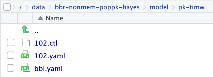
Prior to creating your new Bayes model object with copy_model_as_nmbayes(), your model directory had three files: the FOCE model control stream, its associated .yaml file, and the bbi.yaml configuration file (discussed below).

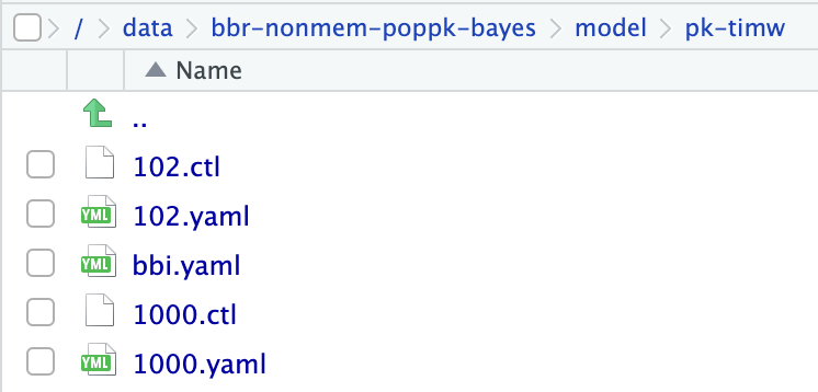
In addition to the new control stream, the copy_model_as_nmbayes() function creates a 1000.yaml file in your model directory that automatically persists any tags, notes, and other model metadata.

While it’s useful to know that this YAML file exists, you shouldn’t need to interact with it directly (e.g., in the RStudio file tabs). Instead, bbr has a variety of functions (i.e., add_tags() and add_notes(), shown below) that work with the model object to edit the information in the YAML file from your R console.

The `bbi.yaml` file

Global settings used by bbr are stored in bbi.yaml (located in your model directory). You can read more in the bbi.yaml configuration file section of the “Getting Started” vignette.

Alternative: create a Bayesian model object from scratch

While the previous example involved creating a new Bayes model based on a previous non-Bayes control stream, we can also create the model from scratch. This assumes we already have the control stream 1000a.ctl in place.

mod1000a <- bbr::new_model(
  file.path(MODEL_DIR, "1000a"),
  .model_type = "nmbayes"
)

From bbr’s perspective, this model is no different to the one we created earlier except this one has no parent model to compare with.

Submitting a model

Now you have a model object, you can submit it to run with bbr::submit_model().

submit_model(
  mod1000,
  .bbi_args = list(threads = 2)
)

Our model’s four chains are now running on two threads each. There are numerous customizations available for submitting models. The following provides detailed information in the bbr documentation and R help: ?submit_model and ?modify_bbi_args.

Monitoring submitted models

For models submitted to the SGE grid (the default), you can use system("qstat -f") to check on your model jobs.

In addition, bbr provides some helper functions that show the head and tail (by default, the first three and last five lines) of specified files and prints them to the console. For example, tail_lst shows the latest status of the .lst files for each of the four chains and, in this case, indicates the chains have finished running.

tail_lst(mod1000)

. ── Chain 1 ─────────────────────────────────────────────────────────────────────

. Sun May 12 08:30:45 EDT 2024
. $PROBLEM 1000
. 
. ...
.  Elapsed postprocess time in seconds:     2.74
.  Elapsed finaloutput time in seconds:     0.29
.  #CPUT: Total CPU Time in Seconds,      215.926
. Stop Time:
. Sun May 12 08:32:14 EDT 2024

. ── Chain 2 ─────────────────────────────────────────────────────────────────────

. Sun May 12 08:30:45 EDT 2024
. $PROBLEM 1000
. 
. ...
.  Elapsed postprocess time in seconds:     2.51
.  Elapsed finaloutput time in seconds:     0.30
.  #CPUT: Total CPU Time in Seconds,      216.661
. Stop Time:
. Sun May 12 08:32:14 EDT 2024

. ── Chain 3 ─────────────────────────────────────────────────────────────────────

. Sun May 12 08:30:45 EDT 2024
. $PROBLEM 1000
. 
. ...
.  Elapsed postprocess time in seconds:     2.97
.  Elapsed finaloutput time in seconds:     0.29
.  #CPUT: Total CPU Time in Seconds,      215.025
. Stop Time:
. Sun May 12 08:32:15 EDT 2024

. ── Chain 4 ─────────────────────────────────────────────────────────────────────

. Sun May 12 08:30:45 EDT 2024
. $PROBLEM 1000
. 
. ...
.  Elapsed postprocess time in seconds:     2.58
.  Elapsed finaloutput time in seconds:     0.29
.  #CPUT: Total CPU Time in Seconds,      216.426
. Stop Time:
. Sun May 12 08:32:13 EDT 2024

Likewise, we can check the tail of the OUTPUT files. Again, these now indicate that the chains have finished running, but during the runs these will display the current iteration number.

tail_output(mod1000)

. ── Chain 1 ─────────────────────────────────────────────────────────────────────

. Model already finished running

. ── Chain 2 ─────────────────────────────────────────────────────────────────────

. Model already finished running

. ── Chain 3 ─────────────────────────────────────────────────────────────────────

. Model already finished running

. ── Chain 4 ─────────────────────────────────────────────────────────────────────

. Model already finished running

Summarize model outputs

Once your model has run, you can start looking at the model outputs and creating diagnostics. The bbr.bayes::read_fit_model() function returns a draws_array object from the posterior package.

draws1000 <- read_fit_model(mod1000)
class(draws1000)

. [1] "draws_nmbayes" "draws_array"   "draws"         "array"

There are many helpful functions provided by the posterior package that allow you to interact with this object. For example, we can generate a summary of the posterior for the THETAs:

posterior::subset_draws(draws1000, variable = "THETA") %>% 
  posterior::summarize_draws()

. # A tibble: 5 × 10
.   variable  mean median     sd    mad    q5   q95  rhat ess_bulk ess_tail
.   <chr>    <dbl>  <dbl>  <dbl>  <dbl> <dbl> <dbl> <dbl>    <dbl>    <dbl>
. 1 THETA[1] 0.475  0.475 0.0646 0.0625 0.369 0.581 1.00      309.     841.
. 2 THETA[2] 4.10   4.10  0.0290 0.0285 4.05  4.15  1.00     1216.    2330.
. 3 THETA[3] 1.10   1.10  0.0337 0.0319 1.05  1.16  0.999    3046.    3457.
. 4 THETA[4] 4.23   4.23  0.0249 0.0246 4.19  4.27  1.00      422.     712.
. 5 THETA[5] 1.30   1.30  0.0368 0.0375 1.24  1.36  1.00      180.     459.

Or we can generate MCMC diagnostic plots by also making use of the bayesplot package:

posterior::subset_draws(draws1000, variable = "THETA") %>% 
  bayesplot::mcmc_trace()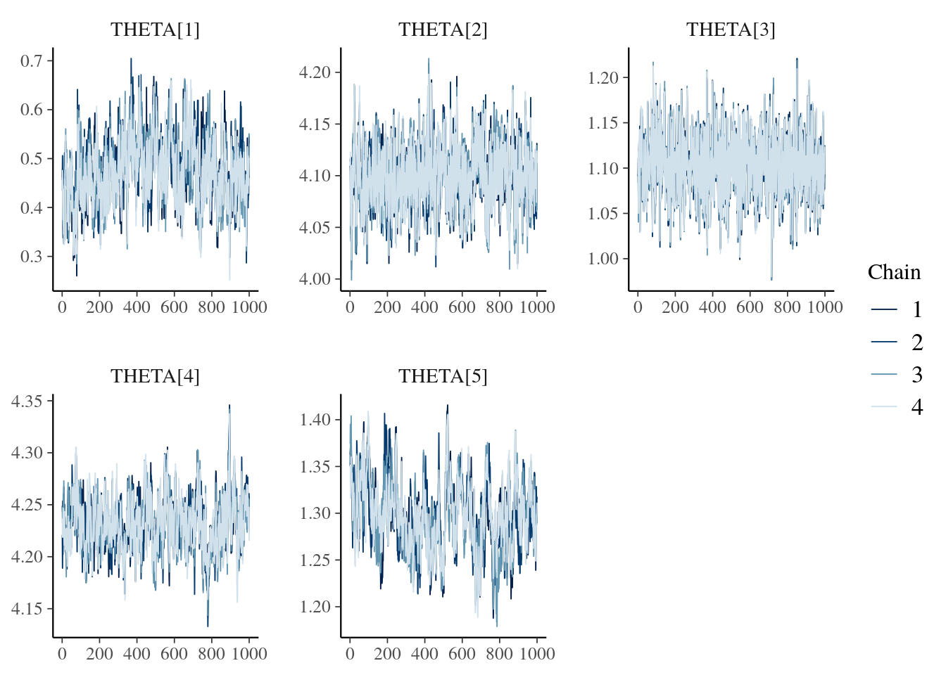

Figure 1: MCMC trace plots for model 1000.

Or we can convert the draws to a data frame to further process the results in other ways:

draws_df <- posterior::as_draws_df(draws1000)
draws_df %>%
  as_tibble() %>% 
  select(starts_with("THETA"), starts_with("."))

. # A tibble: 4,000 × 8
.    `THETA[1]` `THETA[2]` `THETA[3]` `THETA[4]` `THETA[5]` .chain .iteration
.         <dbl>      <dbl>      <dbl>      <dbl>      <dbl>  <int>      <int>
.  1      0.462       4.11       1.09       4.25       1.36      1          1
.  2      0.479       4.10       1.11       4.24       1.37      1          2
.  3      0.395       4.04       1.04       4.25       1.34      1          3
.  4      0.355       4.04       1.07       4.24       1.34      1          4
.  5      0.338       4.06       1.10       4.25       1.35      1          5
.  6      0.405       4.09       1.12       4.25       1.37      1          6
.  7      0.355       4.07       1.10       4.24       1.36      1          7
.  8      0.343       4.02       1.06       4.24       1.35      1          8
.  9      0.375       4.07       1.06       4.26       1.34      1          9
. 10      0.453       4.12       1.15       4.23       1.34      1         10
. # ℹ 3,990 more rows
. # ℹ 1 more variable: .draw <int>

See the posterior package for other helpers.

During model development, MCMC and goodness-of-fit (GOF) diagnostic plots are typically generated to assess model fit. We demonstrate how to make these on the Model Diagnostics, MCMC Diagnostics, and Parameterized Reports for Model Diagnostics pages. Our parameterized reports generate a browsable .html file including the model summary and all MCMC and GOF diagnostic plots (in your model directory). They also save out each plot to .pdf files in deliv/figure/{run}/. You can include any plots of particular interest here, for example, these trace plots:

knitr::include_graphics(file.path(FIGURE_DIR, "1000/1000-mcmc-history.pdf"))

Annotating your model

bbr has some great features that allow you to easily annotate your models. This helps you document your modeling process as you go, and can be easily retrieved later for creating “run logs” that describe the entire analysis. These fields are described in more detail in MeRGE Expo 1. In this example, we make use of these annotations without further explanation.

Based on the output of summarize_draws() above, the following provides an example of how you can add a note to your model, and then move on to testing a model using No-U-Turn Sampler (NUTS) (model 1001 in the next section).

mod1000 <- mod1000 %>% 
  add_notes("Low ESS for some parameters. Try METHOD=NUTS.")

Iterative model development

After running your first model, you can create a new model based on the previous model using the bbr::copy_model_from() function. This will accomplish several objectives:

Copy the control stream associated with .parent_mod and rename it according to .new_model.
Create a new model object associated with this new control stream.
Fill the based_on field in the new model object (see the “Using based_on” vignette).
Optionally, inherit any tags from the parent model.

Using `copy_model_from()`

Learn more about this function from ?copy_model_from or the Iteration section of the “Getting Started” vignette.

mod1001 <- copy_model_from(
    .parent_mod = mod1000,
    .new_model = 1001,
    .inherit_tags = TRUE
  ) %>% 
  replace_tag(TAGS$bayes, TAGS$nuts)

Though .new_model = 1001 is explicitly passed here, this argument can be omitted if naming your models numerically, as in this example. If .new_model is not passed, bbr defaults to incrementing the new model name to the next available integer in the same directory as .parent_mod.

Note that we also update the model tags to reflect the change in estimation method.

Edit your control stream

As mentioned above, you need to manually edit the new control stream with any modifications. In this case, we updated the model structure from one- to -two compartments.

If using RStudio, you can easily open your control stream for editing with the following:

mod1001 %>% open_model_file()

Like before, we use the update_model_id function to update the relevant suffixes in the control stream from “1000” to “1001”.

mod1001 <- update_model_id(mod1001)

You can easily look at the differences between control streams of a model and its parent model:

model_diff(mod1001)

<
 
1001
>
 
1000
@@ 1,3 @@
@@ 1,3 @@
<
 
$PROBLEM From bbr: see 1001.yaml for details
>
 
$PROBLEM 1000
 
 
 
 
 
 
 
 
$INPUT C NUM ID TIME SEQ CMT EVID AMT DV AGE WT HT EGFR ALB BMI SEX AAG
 
 
$INPUT C NUM ID TIME SEQ CMT EVID AMT DV AGE WT HT EGFR ALB BMI SEX AAG
@@ 76,6 @@
@@ 76,6 @@
 
 
$SIGMAPD (1 FIX)
 
 
$SIGMAPD (1 FIX)
 
 
 
 
 
 
<
 
$EST METHOD=CHAIN FILE=1001.chn NSAMPLE=4 ISAMPLE=0 SEED=1 CTYPE=0 IACCEPT=0.3 DF=10 DFS=0
>
 
$EST METHOD=CHAIN FILE=1000.chn NSAMPLE=4 ISAMPLE=0 SEED=1 CTYPE=0 IACCEPT=0.3 DF=10 DFS=0
<
 
$EST METHOD=NUTS AUTO=2 CTYPE=0 OLKJDF=2 OVARF=1 SEED=1 NBURN=250 NITER=500 NUTS_DELTA=0.95 PRINT=10 MSFO=./1001.msf RANMETHOD=P PARAFPRINT=10000 BAYES_PHI_STORE=1
>
 
$EST METHOD=BAYES SEED=1 NBURN=500 NITER=1000 PRINT=10 MSFO=./1000.msf RANMETHOD=P PARAFPRINT=10000 BAYES_PHI_STORE=0
 
 
 
 
 
 
<
 
$TABLE NUM CL V2 Q V3 KA ETAS(1:LAST) EPRED IPRED NPDE EWRES NOPRINT ONEHEADER FILE=1001.tab RANMETHOD=P
>
 
$TABLE NUM CL V2 Q V3 KA ETAS(1:LAST) EPRED IPRED NPDE EWRES NOPRINT ONEHEADER FILE=1000.tab RANMETHOD=P

Submit the model

After manually updating your new control stream, you can submit it to run.

submit_model(
  mod1001,
  .bbi_args = list(threads = 2)
)

Add notes and description

After running model 1001, we consider MCMC diagnostics and standard model diagnostics to be suitable. For example, ESS is suitably high for all parameters and normalized prediction distribution error (NPDE) plots show no reason for concern.

draws1001 <- read_fit_model(mod1001)
posterior::subset_draws(draws1001, variable = "THETA") %>% 
  posterior::summarize_draws()

. # A tibble: 5 × 10
.   variable  mean median     sd    mad    q5   q95  rhat ess_bulk ess_tail
.   <chr>    <dbl>  <dbl>  <dbl>  <dbl> <dbl> <dbl> <dbl>    <dbl>    <dbl>
. 1 THETA[1] 0.479  0.477 0.0625 0.0646 0.377 0.580  1.00    1530.    1522.
. 2 THETA[2] 4.10   4.10  0.0272 0.0282 4.06  4.15   1.00     764.    1283.
. 3 THETA[3] 1.10   1.10  0.0340 0.0331 1.05  1.16   1.00     948.    1275.
. 4 THETA[4] 4.23   4.23  0.0250 0.0256 4.19  4.27   1.00    2081.    1731.
. 5 THETA[5] 1.29   1.29  0.0379 0.0377 1.23  1.35   1.00    2204.    1620.

knitr::include_graphics(file.path(FIGURE_DIR, "1001/1001-npde-pred-time-tad.pdf"))

Thus, we add a note to the model to indicate this, and add a description to denote mod1001 as the final base model.

mod1001 <- mod1001 %>% 
  add_notes("All diagnostics look reasonable") %>% 
  add_description("Final base model")

Final model

Including covariate effects

After identifying our base model, we copy the base model, add some pre-specified covariates to the control stream to create our full covariate model, and include tags to indicate the covariates added:

mod1100 <- copy_model_from(
    mod1001,
    1100,
    .inherit_tags = TRUE
  ) %>% 
  add_tags(c(
    TAGS$cov_cl_egfr,
    TAGS$cov_cl_age,
    TAGS$cov_cl_alb
  ))

Remember to edit the control stream manually:

model_diff(mod1100)

<
 
1100
>
 
1001
@@ 1,3 @@
@@ 1,3 @@
<
 
$PROBLEM From bbr: see 1100.yaml for details
>
 
$PROBLEM From bbr: see 1001.yaml for details
 
 
 
 
 
 
 
 
$INPUT C NUM ID TIME SEQ CMT EVID AMT DV AGE WT HT EGFR ALB BMI SEX AAG
 
 
$INPUT C NUM ID TIME SEQ CMT EVID AMT DV AGE WT HT EGFR ALB BMI SEX AAG
@@ 11,8 @@
@@ 11,4 @@
 
 
 
 
 
 
 
 
;log transformed PK parms
 
 
;log transformed PK parms
<
 
 
~
 
<
 
  CLEGFR = LOG(EGFR/90) * THETA(6)
~
 
<
 
  CLAGE  = LOG(AGE/35) * THETA(7)
~
 
<
 
  CLALB  = LOG(ALB/4.5) * THETA(8)
~
 
 
 
 
 
 
 
 
 
  V2WT   = LOG(WT/70)
 
 
  V2WT   = LOG(WT/70)
@@ 23,7 @@
@@ 19,9 @@
 
 
  MU_1   = THETA(1)
 
 
  MU_1   = THETA(1)
 
 
  MU_2   = THETA(2) + V2WT
 
 
  MU_2   = THETA(2) + V2WT
<
 
  MU_3   = THETA(3) + CLWT + CLEGFR + CLAGE + CLALB
>
 
  MU_3   = THETA(3) + CLWT
 
 
  MU_4   = THETA(4) + V3WT
 
 
  MU_4   = THETA(4) + V3WT
 
 
  MU_5   = THETA(5) + QWT
 
 
  MU_5   = THETA(5) + QWT
~
 
>
 
 
~
 
>
 
  ;" CALL EXTRASEND()
 
 
 
 
 
 
 
 
  KA     = EXP(MU_1 + ETA(1))
 
 
  KA     = EXP(MU_1 + ETA(1))
@@ 47,7 @@
@@ 45,4 @@
 
 
  (4)     ; 4 V3 (L) - 70
 
 
  (4)           ; 4 V3 (L) - 70
 
 
  (2)     ; 5 Q  (L/hr) - 4
 
 
  (2)           ; 5 Q  (L/hr) - 4
<
 
  (1)     ; 6 CLEGFR~CL ()
~
 
<
 
  (1)     ; 7 AGE~CL ()
~
 
<
 
  (0.5)   ; 8 ALB~CL ()
~
 
 
 
 
 
 
 
 
 
$OMEGA BLOCK(3)
 
 
$OMEGA BLOCK(3)
@@ 70,8 @@
@@ 65,5 @@
 
 
  (4)   FIX      ; 4 V3 (L) - 70
 
 
  (4)   FIX        ; 4 V3 (L) - 70
 
 
  (2)   FIX      ; 5 Q  (L/hr) - 4
 
 
  (2)   FIX        ; 5 Q  (L/hr) - 4
<
 
  (1)   FIX   ; 6 CLEGFR~CL ()
~
 
<
 
  (1)   FIX   ; 7 AGE~CL ()
~
 
<
 
  (0.5) FIX   ; 8 ALB~CL ()
~
 
<
 
$THETAPV BLOCK(8) VALUES(10, 0) FIX
>
 
$THETAPV BLOCK(5) VALUES(10, 0) FIX
 
 
 
 
 
 
 
 
$OMEGAP BLOCK(3) VALUES(0.2, 0.01) FIX
 
 
$OMEGAP BLOCK(3) VALUES(0.2, 0.01) FIX
@@ 84,6 @@
@@ 76,6 @@
 
 
$SIGMAPD (1 FIX)
 
 
$SIGMAPD (1 FIX)
 
 
 
 
 
 
<
 
$EST METHOD=CHAIN FILE=1100.chn NSAMPLE=4 ISAMPLE=0 SEED=1 CTYPE=0 IACCEPT=0.3 DF=10 DFS=0
>
 
$EST METHOD=CHAIN FILE=1001.chn NSAMPLE=4 ISAMPLE=0 SEED=1 CTYPE=0 IACCEPT=0.3 DF=10 DFS=0
<
 
$EST METHOD=NUTS AUTO=2 CTYPE=0 OLKJDF=2 OVARF=1 SEED=1 NBURN=250 NITER=500 NUTS_DELTA=0.95 PRINT=10 MSFO=./1100.msf RANMETHOD=P PARAFPRINT=10000 BAYES_PHI_STORE=1
>
 
$EST METHOD=NUTS AUTO=2 CTYPE=0 OLKJDF=2 OVARF=1 SEED=1 NBURN=250 NITER=500 NUTS_DELTA=0.95 PRINT=10 MSFO=./1001.msf RANMETHOD=P PARAFPRINT=10000 BAYES_PHI_STORE=1
 
 
 
 
 
 
<
 
$TABLE NUM CL V2 Q V3 KA ETAS(1:LAST) EPRED IPRED NPDE EWRES NOPRINT ONEHEADER FILE=1100.tab RANMETHOD=P
>
 
$TABLE NUM CL V2 Q V3 KA ETAS(1:LAST) EPRED IPRED NPDE EWRES NOPRINT ONEHEADER FILE=1001.tab RANMETHOD=P

We are now ready to submit the model.

submit_model(
  mod1100,
  .bbi_args = list(threads = 2)
)

Choose final model

After checking your model heuristics, parameter estimates, and GOF plots, the final model was determined to be run 1100. As above, this model can be identified as the “final model” in the description field so it can easily be identified as a key model when looking at the run log later.

mod1100 <- mod1100 %>%
  add_notes("All diagnostics look reasonable") %>% 
  add_description("Final Model")

Submit models to be re-run

There are cases when some or all of your models need to be re-run. For example, maybe your model or data files changed since the model was last run.

You can check whether any changes have been made to the model or data since the last time the model was run using either the bbr::config_log() function or with bbr functions that track model lineage; examples of both approaches are shown in the “Using the based_on field” vignette.

To re-run a single model, simply pass .overwrite = TRUE to the submit_model() call.

submit_model(mod1000, .overwrite=TRUE)

Other resources

The following scripts from the GitHub repository are discussed on this page. If you’re interested running this code, visit the About the GitHub Repo page first.

Model management “scratch pad” script: model-management.R
Runnable version of the examples on this page: model-management-demo.Rmd

Model Management

Introduction

Tools used

MetrumRG packages

CRAN packages

Outline

Set up

Model creation and submission

Previous FOCE model

Copy FOCE model to a Bayesian model object

Edit your control stream

The model YAML file

The `bbi.yaml` file

Alternative: create a Bayesian model object from scratch

Submitting a model

Monitoring submitted models

Summarize model outputs

Annotating your model

Iterative model development

Using `copy_model_from()`

Edit your control stream

Submit the model

Add notes and description

Final model

Including covariate effects

Choose final model

Submit models to be re-run

Other resources

More `bbr` resources

Introduction

Tools used

MetrumRG packages

CRAN packages

Outline

Set up

Model creation and submission

Previous FOCE model

Copy FOCE model to a Bayesian model object

Edit your control stream

The model YAML file

The bbi.yaml file

Alternative: create a Bayesian model object from scratch

Submitting a model

Monitoring submitted models

Summarize model outputs

Annotating your model

Iterative model development

Using copy_model_from()

Edit your control stream

Submit the model

Add notes and description

Final model

Including covariate effects

Choose final model

Submit models to be re-run

Other resources

More bbr resources

The `bbi.yaml` file

Using `copy_model_from()`

More `bbr` resources