1100.The final covariate model included the following features:
Two compartment disposition parameterized in terms of:
First-order absorption (KA)
First-order elimination
Allometric scaling- clearances and volumes
Covariate effects
Subject-level random effects
Proportional residual error
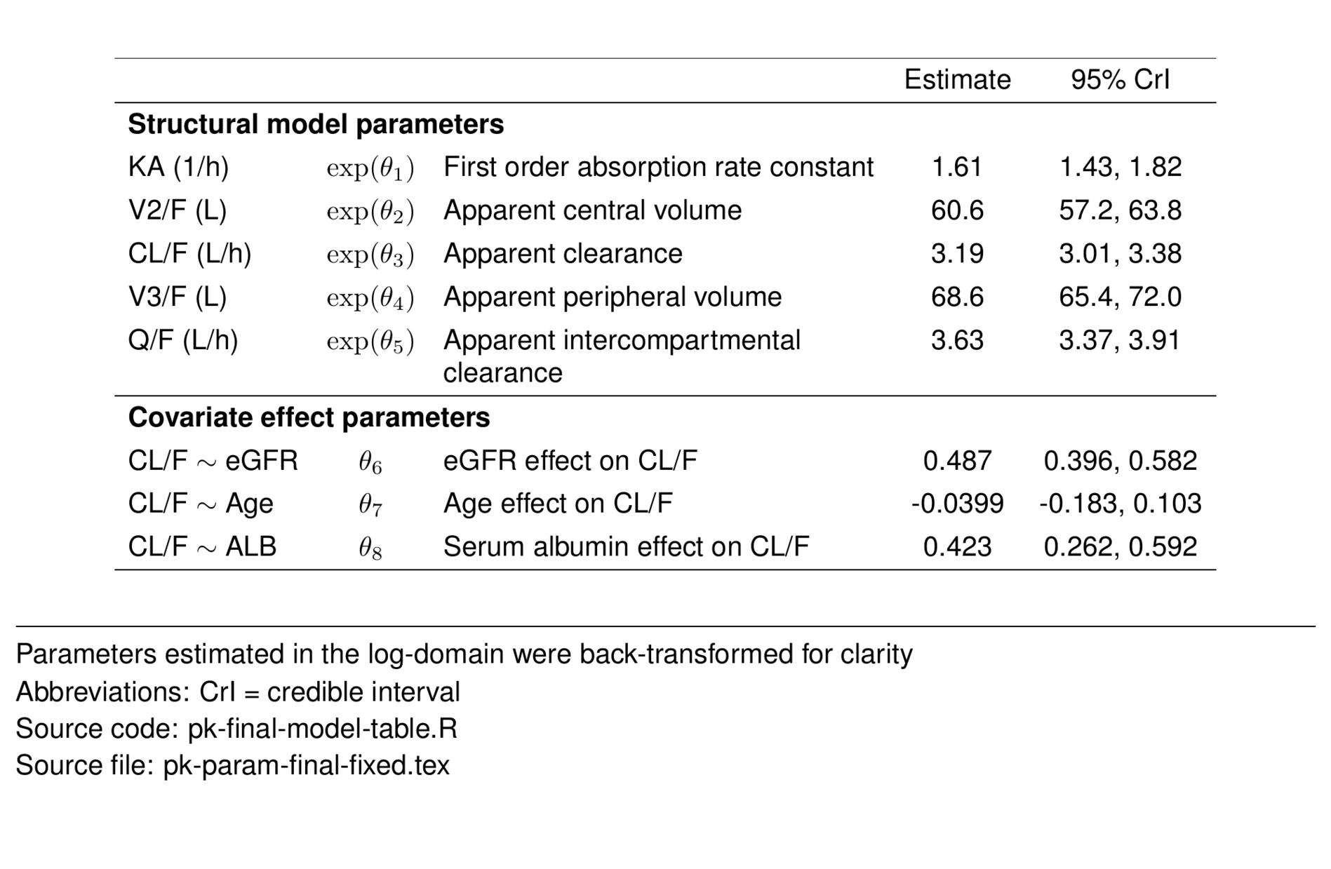
The final model included fixed effects of body weight on all CL/F and V/F terms. Additionally, the effects of age, eGFR, and albumin were estimated on drug CL/F.
\[ CL/F_i = e^{(\theta_{3} + \text{WT}_\mathit{CL/F} + \text{EGFR}_\mathit{CL/F} + \text{AGE}_\mathit{CL/F} + \text{ALB}_\mathit{CL/F} + \eta_{3i})} \]
\[ \mathit{V2/F_i}=e^{(\theta_{2} + \text{WT}_{V/F} + \eta_{2i})} \\ \] \[ \mathit{Q/F_i}=e^{(\theta_{5} + \text{WT}_{Q/F})} \] \[ \mathit{V3/F_i}=e^{(\theta_{4} + \text{WT}_{V/F})} \]
\[ \mathit{KA_i}=e^{(\theta_{1} + \eta_{1i})} \\ \]
where
\[ \text{WT}_\mathit{CL/F} = 0.75 \cdot \log\big(\text{WT}_i/70\big) \]
\[ \text{EGFR}_\mathit{CL/F} = \theta_6 \cdot \log\big(\text{EGFR}_i/90\big) \]
\[ \text{AGE}_\mathit{CL/F} = \theta_7 \cdot \log\big(\text{AGE}_i/35\big) \]
\[ \text{ALB}_\mathit{CL/F} = \theta_8 \cdot \log\big(\text{ALB}_i/4.5\big) \]
\[ \text{WT}_\mathit{V/F} = 1.00 \cdot \log\big(\text{WT}_i/70\big) \]
\[ \text{WT}_\mathit{Q/F} = 0.75 \cdot \log\big(\text{WT}_i/70\big) \]
\[ Y_\mathit{i,y} = \widehat{Y_\mathit{i,j}} \cdot \big(1+\varepsilon_\mathit{i,j}\big) \]
where
Models were fit with weakly-informative priors. The NONMEM® $PRIOR NWPRI subroutine was used to select normal distribution priors for THETAs and inverse Wishart distribution priors for SIGMAs. Variances of 10 were used for all THETA priors (with parameters estimated on the log scale), and the degrees of freedom for OMEGA and SIGMA priors were 3 and 1, respectively, corresponding to the block size of each matrix.
1100.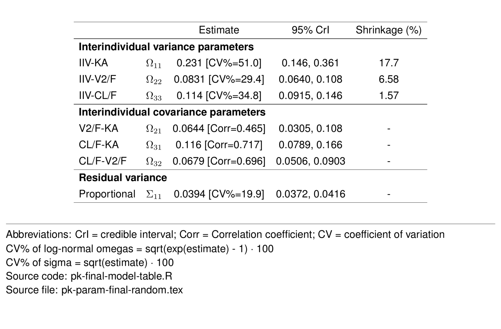
1100.library(mrgsolve)
library(dplyr)
library(here)
library(ggplot2)
library(forcats)
library(patchwork)
theme_set(theme_bw())
mod <- mread(here("script/model/1100.mod")) %>% zero_re()
data <- as_data_set(
evd(amt = 25),
evd(amt = 25, ii = 24, addl = 10)
)
out <- mrgsim(mod, data, output = "df", delta = 0.1, end = 480)
out <- mutate(
out,
lbl = case_when(
ID==1 ~ "Single dose",
ID==2 ~ "Multiple dose, q24h x10"
),
lbl = forcats::fct_inorder(lbl)
)
b <- filter(out, ID==2)
a <- filter(out, ID==1 & TIME <= 96)
pa <- ggplot(a) +
geom_line(aes(TIME, Y)) +
facet_wrap(~lbl, scales = "free_x") +
labs(x = "Time (hours)", y = "Concentration (ng/mL)") +
scale_x_continuous(breaks = seq(0,96,8)) +
scale_y_continuous(limits = c(0, 600))
pb <-
ggplot(b) +
geom_line(aes(TIME/24, Y)) +
facet_wrap(~lbl, scales = "free_x") +
labs(x = "Time (days)", y = "") +
scale_x_continuous(breaks = seq(0,20,2)) +
scale_y_continuous(limits = c(0, 600))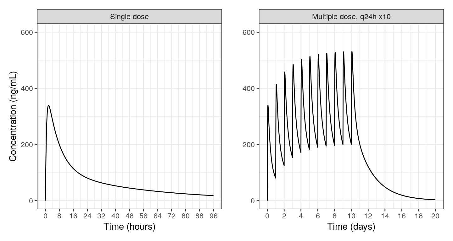
$PROBLEM From bbr: see 1100.yaml for details

$INPUT C NUM ID TIME SEQ CMT EVID AMT DV AGE WT HT EGFR ALB BMI SEX AAG
  SCR AST ALT CP TAFD TAD LDOS MDV BLQ PHASE

$DATA ../../../data/derived/pk.csv IGNORE=(C='C', BLQ=1)

$SUBROUTINE ADVAN4 TRANS4

$PK

;log transformed PK parms

  CLEGFR = LOG(EGFR/90) * THETA(6)
  CLAGE  = LOG(AGE/35) * THETA(7)
  CLALB  = LOG(ALB/4.5) * THETA(8)

  V2WT   = LOG(WT/70)
  CLWT   = LOG(WT/70) * 0.75
  V3WT   = LOG(WT/70)
  QWT    = LOG(WT/70) * 0.75

  MU_1   = THETA(1)
  MU_2   = THETA(2) + V2WT
  MU_3   = THETA(3) + CLWT + CLEGFR + CLAGE + CLALB
  MU_4   = THETA(4) + V3WT
  MU_5   = THETA(5) + QWT

  KA     = EXP(MU_1 + ETA(1))
  V2     = EXP(MU_2 + ETA(2))
  CL     = EXP(MU_3 + ETA(3))
  V3     = EXP(MU_4 + ETA(4))
  Q      = EXP(MU_5 + ETA(5))

  S2     = V2/1000 ; dose in mcg, conc in mcg/mL

$ERROR

  IPRED = F
  Y     = IPRED * (1 + EPS(1))

$THETA
; log values
  (0.5)   ; 1 KA (1/hr) - 1.5
  (3.5)   ; 2 V2 (L) - 60
  (1)     ; 3 CL (L/hr) - 3.5
  (4)     ; 4 V3 (L) - 70
  (2)     ; 5 Q  (L/hr) - 4
  (1)     ; 6 CLEGFR~CL ()
  (1)     ; 7 AGE~CL ()
  (0.5)   ; 8 ALB~CL ()

$OMEGA BLOCK(3)
  0.2           ; ETA(KA)
  0.01 0.2      ; ETA(V2)
  0.01 0.01 0.2 ; ETA(CL)
$OMEGA
  0.025 FIX    ; ETA(V3)
  0.025 FIX    ; ETA(Q)

$SIGMA
  0.05          ; 1 pro error

$PRIOR NWPRI

$THETAP
  (0.5) FIX      ; 1 KA (1/hr) - 1.5
  (3.5) FIX      ; 2 V2 (L) - 60
  (1)   FIX      ; 3 CL (L/hr) - 3.5
  (4)   FIX      ; 4 V3 (L) - 70
  (2)   FIX      ; 5 Q  (L/hr) - 4
  (1)   FIX   ; 6 CLEGFR~CL ()
  (1)   FIX   ; 7 AGE~CL ()
  (0.5) FIX   ; 8 ALB~CL ()
$THETAPV BLOCK(8) VALUES(10, 0) FIX

$OMEGAP BLOCK(3) VALUES(0.2, 0.01) FIX

$OMEGAPD (3 FIX)

$SIGMAP
  0.05 FIX           ; 1 pro error

$SIGMAPD (1 FIX)

$EST METHOD=CHAIN FILE=1100.chn NSAMPLE=4 ISAMPLE=0 SEED=1 CTYPE=0 IACCEPT=0.3 DF=10 DFS=0
$EST METHOD=NUTS AUTO=2 CTYPE=0 OLKJDF=2 OVARF=1 SEED=1 NBURN=250 NITER=500 NUTS_DELTA=0.95 PRINT=10 MSFO=./1100.msf RANMETHOD=P PARAFPRINT=10000 BAYES_PHI_STORE=1

$TABLE NUM CL V2 Q V3 KA ETAS(1:LAST) EPRED IPRED NPDE EWRES NOPRINT ONEHEADER FILE=1100.tab RANMETHOD=P[ prob ]
1100
[ pkmodel ] cmt = "GUT,CENT,PERIPH", depot = TRUE
[ param ]
WT = 70
EGFR = 90
AGE = 35
ALB = 4.5
[ nmext ]
path = '../../model/pk/1100/1100-1/1100-1.ext'
root = 'cppfile'
[ main ]
double CLEGFR = log(EGFR/90) * THETA6;
double CLAGE = log(AGE/35) * THETA7;
double CLALB = log(ALB/4.5) * THETA8;
double V2WT = log(WT/70);
double CLWT = log(WT/70) * 0.75;
double V3WT = log(WT/70);
double QWT = log(WT/70) * 0.75;
capture KA = exp(THETA1 + ETA(1));
capture V2 = exp(THETA2 + V2WT + ETA(2));
capture CL = exp(THETA3 + CLWT + CLEGFR + CLAGE + CLALB + ETA(3));
capture V3 = exp(THETA4 + V3WT + ETA(4));
capture Q = exp(THETA5 + QWT + ETA(5));
double S2 = V2/1000; //; dose in mcg, conc in mcg/mL
[ table ]
capture IPRED = CENT/S2;
capture Y = IPRED * (1 + EPS(1));