library(bbr)
library(bbr.bayes)
library(dplyr)
library(here)
library(tidyverse)
library(yspec)
library(posterior)
library(bayesplot)

MODEL_DIR <- here("model", "pk")

bayesplot::color_scheme_set('viridis')
theme_set(theme_bw())Introduction
In this expo, we make the distinction between two types of diagnostics:
- Markov Chain Monte Carlo (MCMC) convergence diagnostics
- Model diagnostics, aka goodness-of-fit (GOF) diagnostics
This page demonstrates the use of bbr.bayes, and other tools, to generate MCMC diagnostics for NONMEM® Bayesian (Bayes) models.
There is no explicit functionality in bbr.bayes to perform these steps; however, the output from bbr.bayes makes these steps relatively simple.
See the end of this page for a video overview of content covered here.
Tools used
MetrumRG packages
bbr Manage, track, and report modeling activities, through simple R objects, with a user-friendly interface between R and NONMEM®.
bbr.bayes Extension of the bbr package to support Bayesian modeling with Stan or NONMEM®.
CRAN packages
dplyr A grammar of data manipulation.
bayesplot Plotting Bayesian models and diagnostics with ggplot.
posterior Provides tools for working with output from Bayesian models, including output from CmdStan.
Set up
Load required packages and set file paths to your model and figure directories.
MCMC diagnostics
After fitting the model, we examine a suite of MCMC diagnostics to see if anything is amiss with the sampling. We’ll focus on split R-hat, bulk and tail ESS, trace plots, and density plots. If any of these raise a flag about convergence, then additional diagnostics would be examined.
Model summary
We begin by reading in the output from our first base model, run 1000. This is done using the read_fit_model function from bbr.bayes, which returns a draws_array object from the posterior package.
model_name <- 1000
draws <- read_fit_model(file.path(MODEL_DIR, model_name))
n_chains <- nchains(draws)
n_iter <- niterations(draws)

draws_param <- subset_draws(draws, variable = c("THETA", "OMEGA", "SIGMA"))
draws_sum <- draws_param %>%  summarize_draws()

fixed <- is.na(draws_sum$rhat)
pars <- variables(draws_param)[!fixed]
draws_sum %>%
  filter(variable %in% pars) %>%
  mutate(across(-variable, ~ pmtables::sig(.x, maxex = 4)))
. # A tibble: 12 × 10
. variable mean median sd mad q5 q95 rhat ess_bulk ess_tail
. <chr> <chr> <chr> <chr> <chr> <chr> <chr> <chr> <chr> <chr>
. 1 THETA[1] 0.475 0.475 0.0646 0.0625 0.369 0.581 1.00 309 841
. 2 THETA[2] 4.10 4.10 0.0290 0.0285 4.05 4.15 1.00 1220 2330
. 3 THETA[3] 1.10 1.10 0.0337 0.0319 1.05 1.16 0.999 3050 3460
. 4 THETA[4] 4.23 4.23 0.0249 0.0246 4.19 4.27 1.00 422 712
. 5 THETA[5] 1.30 1.30 0.0368 0.0375 1.24 1.36 1.00 180 459
. 6 OMEGA[1,1] 0.257 0.251 0.0595 0.0564 0.171 0.366 1.01 363 771
. 7 OMEGA[2,1] 0.0774 0.0758 0.0224 0.0219 0.0440 0.117 1.01 614 1450
. 8 OMEGA[2,2] 0.0903 0.0894 0.0127 0.0125 0.0714 0.112 1.01 1460 2510
. 9 OMEGA[3,1] 0.138 0.137 0.0277 0.0279 0.0962 0.186 1.00 1030 2260
. 10 OMEGA[3,2] 0.0747 0.0739 0.0133 0.0131 0.0542 0.09… 1.00 1950 2320
. 11 OMEGA[3,3] 0.176 0.175 0.0203 0.0201 0.144 0.210 0.999 3240 3700
. 12 SIGMA[1,1] 0.0394 0.0394 0.00111 0.00115 0.0376 0.04… 1.00 2790 3530For the population-level parameters, the R-hat values are all below 1.01. But, some ESS bulk and tail values are on the low side, particularly for THETA5 (intercompartmental clearance, Q).
R-hat plot
We can visualize the R-hat values with the mcmc_rhat function from bayesplot.
rhats <- draws_sum$rhat
names(rhats) <- draws_sum$variable
rhat_plot <- mcmc_rhat(rhats, pars = pars) + yaxis_text()
rhat_plot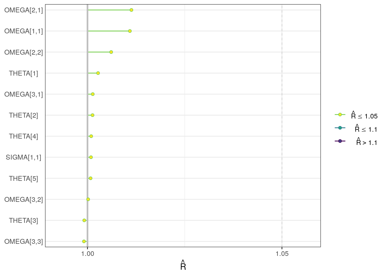
ESS plots
We can also visualize the bulk and tail ESS as ratios of the effective sample size (Neff) to the total number of iterations (N). Further ESS plots are included in template-mcmc.Rmd.
ess_bulk <- draws_sum$ess_bulk
names(ess_bulk) <- draws_sum$variable
ess_bulk_ratios <- ess_bulk / (n_iter * n_chains)
ess_bulk_plot <- mcmc_neff(ess_bulk_ratios) + yaxis_text() +
  labs(title = "Bulk ESS ratios")
ess_bulk_plot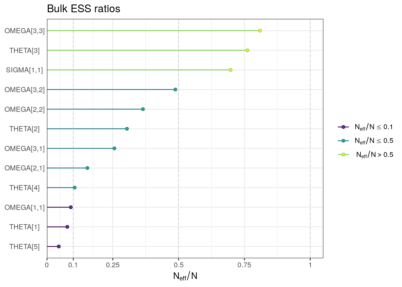
ess_tail <- draws_sum$ess_tail
names(ess_tail) <- draws_sum$variable
ess_tail_ratios <- ess_tail / (n_iter * n_chains)
ess_tail_plot <- mcmc_neff(ess_tail_ratios) + yaxis_text() +
  labs(title = "Tail ESS ratios")
ess_tail_plot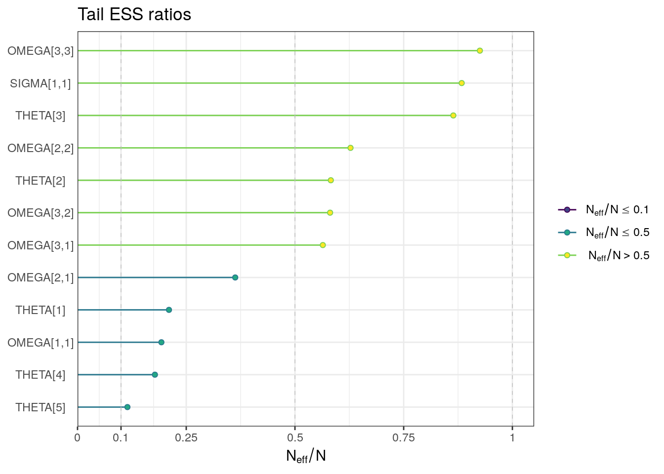
Trace and density plots
Next, we look at the trace and density plots.
trace0 <- mcmc_trace(draws, pars = pars)trace0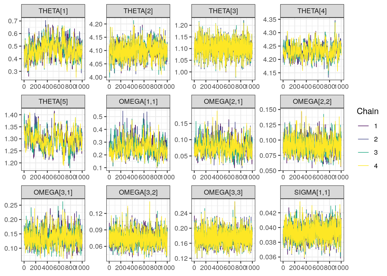
density0 <- mcmc_dens_overlay(draws, pars = pars)density0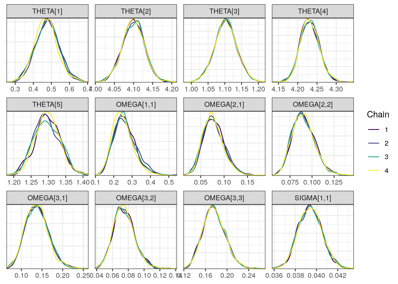
A scatterplot of the MCMC draws can be useful in showing bivariate relationships in the posterior distribution. The default scatterplot generated with mcmc_pairs uses points for the off-diagonal panels and histograms along the diagonal. We restrict this plot to only the THETAs to keep the size manageable.
mcmc_pairs(draws, regex_pars = "THETA")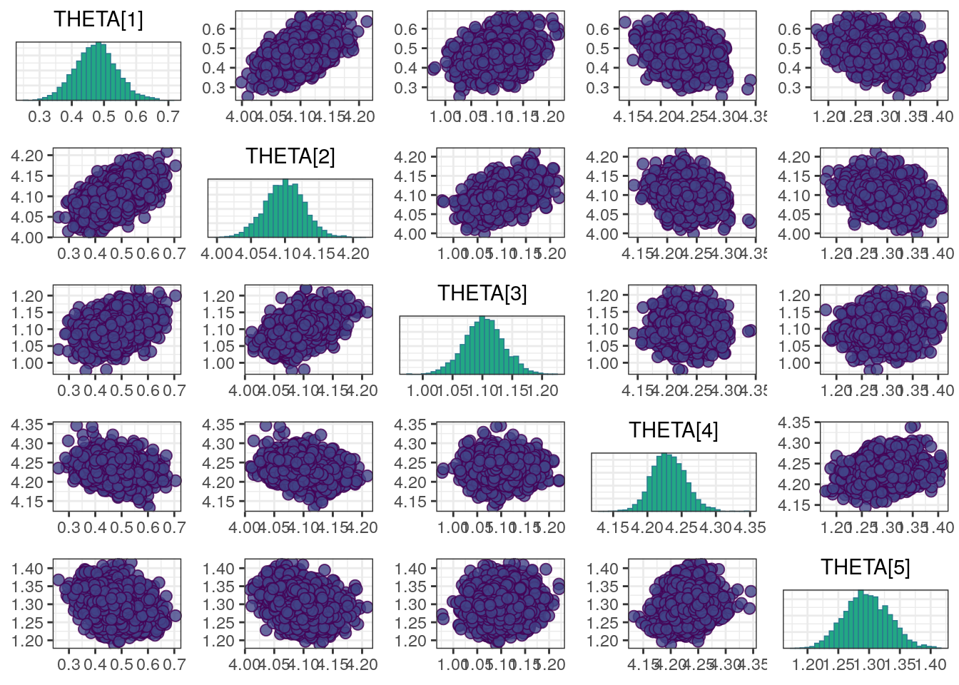
Although all R-hat values are low and scatterplots reasonable, some ESS values are on the low side which corresponds to some trace plots resembling “wiggly worms” than “fuzzy caterpillars.
Other resources
The following script from the GitHub repository is discussed on this page. If you’re interested running this code, visit the About the GitHub Repo page first.
MCMC Diagnostics template: template-mcmc.Rmd
More details on the visual MCMC diagnostics are available in a Vignettes from bayesplot package developers.