library(pmforest)
library(tidyverse)
library(mrgsolve)
library(here)
library(yspec)
library(glue)
library(rlang)
library(bbr)
library(bbr.bayes)
library(posterior)Introduction
This page demonstrates how to use the pmforest package along with mrgsolve to create covariate forest plots. These plots provide context around estimated covariate effects by simulating model parameters (e.g., clearance) after varying the values of different covariates one at a time. The simulated parameters are normalized to parameters simulated at the reference covariate levels and all simulations are performed over the uncertainty distribution of the THETAs from the estimated model. Sample from the Bayesian (Bayes) posterior are used to represent the uncertainty of THETA estimates.
Tools used
MetrumRG packages
CRAN packages
posterior Provides tools for working with output from Bayesian models, including output from CmdStan.
Outline
First, we load:
- data specification object
- relevant
mrgsolvemodel - data frame of the posterior of parameter estimates
Then, we use the mrgsolve model to simulate clearance parameters across the posterior parameter estimate set for the reference covariate set.
Next, we simulate clearances (again across the posterior parameter set) after varying the values of the different model covariates one at a time. This illustrates how changes in the covariate translate into changes in clearance.
Finally, we summarize the simulated clearance values at each covariate level and create a forest plot from these summarized simulations.
Required packages and options
Load the data specification object
Load the yspec object, this provides information about the data set (including model covariates):
spec <- ys_load(here("data/derived/pk.yml"))We can include units on the plots (by pulling them from the spec), but we can also modify units to be blank:
spec$EGFR$unit <- ""Then, extract a list of units to annotate the plot:
unit <-
  spec %>%
  ys_get_unit() %>%
  as_tibble() %>%
  pivot_longer(everything(), values_to = "unit")

head(unit)
# A tibble: 6 × 2
name unit
<chr> <chr>
1 C ""
2 NUM ""
3 ID ""
4 TIME "hour"
5 SEQ ""
6 CMT "" Read in posterior of parameter estimates
The as_draws_df function from the posterior package gives us a draws_df object. We use subset_draws from the posterior package to subset the draws for our purposes.
run <- 1100
MODEL_DIR <- here("model/pk")
mod_bbr <- read_model(file.path(MODEL_DIR, run))
draws <- as_draws_df(mod_bbr)
post <- draws %>%
  subset_draws(variable = c("THETA")) %>%
  as_tibble() %>%
  mutate(iter = row_number()) %>%
  rename_with(~ str_remove_all(.x, "[[:punct:]]"), .cols = starts_with("THETA"))
Read in the mrgsolve model
For the final model (run 1100), we already have the simulation model coded up: 1100.mod . This enables us to simulate clearances from different covariate values.
mod <- mread(here(glue("script/model/{run}.mod")), end = -1, outvars = "CL")

mod <- zero_re(mod)
Note, that we call zero_re() on the model object; this suppresses the simulation of random effects. In this task, we are only interested in simulating typical parameters.
Simulate
Simulate the reference
Simulate a dataframe of clearances at the reference covariate combination:
ref <- mrgsim(mod, idata = post) %>% select(iter = ID, ref = CL)

head(ref)
# A tibble: 6 × 2
iter ref
<dbl> <dbl>
1 1 3.21
2 2 3.21
3 3 3.29
4 4 3.28
5 5 3.19
6 6 3.23Note that this simulation produces clearances at the reference covariate levels because we coded the default covariates to be the reference values in the mrgsolve model.
Simulate different covariate levels
Now, we have to simulate clearances after perturbing each covariate across levels of interest one at a time.
To do this, we create a named list of vectors where the name reflects the covariate being perturbed, and the vector has all the values to examine.
x <- list(
  WT = c(85, 55),
  EGFR = c(Severe = 22.6, Moderate = 42.9, Mild = 74.9),
  ALB = c(5, 3.25),
  AGE = c(45, 20)
)
For EGFR, we’ve included names for recoding the EGFR as a renal impairment stage (e.g., moderate renal impairment).
Now, we write a function that simulates each covariate at each of the prescribed levels:
ss <- function(values, col) {

  COL <- sym(col)

  idata <- tibble(!!COL := values, LVL = seq_along(values))
  idata <- crossing(post, idata)

  out <-
    mod %>%
    mrgsim_i(idata, carry_out = c(col, "LVL", "iter")) %>%
    mutate(name = col, value = !!COL,  !!COL := NULL) %>%
    arrange(LVL)

  if(is_named(values)) {
    out <- mutate(
      out,
      value := factor(value, labels = names(values), levels=values)
    )
  } else {
    out <- mutate(out, value = fct_inorder(as.character(value)))
  }
  out
}
This function gets called using an imap variant to simulate clearances:
out <- imap_dfr(x, ss)
head(out)
# A tibble: 6 × 7
ID time LVL iter CL name value
<dbl> <dbl> <dbl> <dbl> <dbl> <chr> <fct>
1 2 0 1 46 3.46 WT 85
2 4 0 1 1485 3.43 WT 85
3 6 0 1 1484 3.44 WT 85
4 8 0 1 460 3.62 WT 85
5 10 0 1 1483 3.45 WT 85
6 12 0 1 268 3.49 WT 85 This function:
- Creates an
idata_setwith the current covariate name and values - Uses
tidyr::crossingto expandidatato include all the posterior samples loaded frompost - Simulates the clearance
- Post simulation, logs the
nameof the covariate and thevalues simulated - Post simulation, checks whether covariate names were passed and, if so, recodes the covariate values accordingly
The result of the function is 200 clearance values simulated at multiple levels of multiple covariates.
count(out, name, value)# A tibble: 9 × 3
name value n
<chr> <fct> <int>
1 AGE 45 2000
2 AGE 20 2000
3 ALB 5 2000
4 ALB 3.25 2000
5 EGFR Severe 2000
6 EGFR Moderate 2000
7 EGFR Mild 2000
8 WT 85 2000
9 WT 55 2000Plot
Get ready to plot
Merge the units to the model output by name:
out <- left_join(out, unit, by = "name")
out <- mutate(out, cov_level = str_trim(paste(value, unit)))
Merge in the reference clearance values by iter and calculate the simulated clearance relative to the reference (relcl):
out <- left_join(out, ref, by = "iter")
out <- mutate(out, relcl = CL/ref)
Set up labels and create a labeller object:
all_labels <- ys_get_short(spec, title_case = TRUE)
all_labels$EGFR <- 'Renal Function'
all_labels$CL <- 'CL (L/hr)'

plot_labels <- as_labeller(unlist(all_labels))
Summarize the data
Call summarize_data from the pmforest package to generate summaries. Here, we use the 2.5th and 97.5th percentiles of the clearance at each covariate level. summarize_data also returns the median for plotting.
sum_data <- summarize_data(
  data = out,
  value = "relcl",
  group = "name",
  group_level = "cov_level",
  probs = c(0.025, 0.975),
  statistic = "median"
)

head(sum_data)
# A tibble: 6 × 5
group group_level mid lo hi
<chr> <chr> <dbl> <dbl> <dbl>
1 AGE 20 years 1.02 0.944 1.11
2 AGE 45 years 0.990 0.955 1.03
3 ALB 3.25 g/dL 0.871 0.825 0.918
4 ALB 5 g/dL 1.05 1.03 1.06
5 EGFR Mild 0.914 0.899 0.930
6 EGFR Moderate 0.697 0.650 0.745Create the plot
Please see the ?plot_forest documentation for details around each argument.
clp <- plot_forest(
  data = sum_data,
  summary_label = plot_labels,
  text_size = 3.5,
  vline_intercept = 1,
  x_lab = "Fraction and 95% CI \nRelative to Reference",
  CI_label = "Median [95% CI]",
  plot_width = 8,
  x_breaks = c(0.4,0.6, 0.8, 1, 1.2, 1.4,1.6),
  x_limit = c(0.4,1.45),
  annotate_CI = T,
  nrow = 1
)
clp 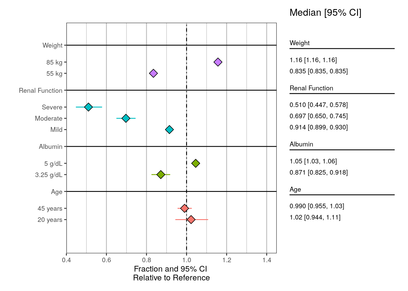
Other resources
The following script from the GitHub repository is discussed on this page. If you’re interested running this code, visit the About the GitHub Repo page first.