library(bbr)
library(bbr.bayes)
library(dplyr)
library(pmplots)
library(here)
library(yspec)
library(glue)
library(patchwork)

library(mrgmisc)
library(yaml)
library(knitr)
library(pmtables)Introduction
During Bayesian (Bayes) model development, we consider two types of diagnostics: Markov chain Monte Carlo (MCMC) convergence diagnostics specific to Bayes models and goodness-of-fit (GOF) diagnostic plots. Here, we demonstrate the latter: generating model GOF diagnostic plots using the pmplots and yspec packages. For information on which diagnostics are most appropriate for your project and how to interpret them, please refer to the Other resources section at the bottom of this page.
The process and tools are similar to those described in the Model Diagnostics of MeRGE Expo 1 (FOCE methods). The main difference here is the use of the nm_join_bayes function from bbr.bayes to generate predicted (EPRED, IPRED), Expected Weight Residuals (EWRES), and Normalized Prediction Distribution Error (NPDE) values from the full Bayes posterior. The reasons for using the full posterior distribution (rather that using the values output in tables) are described here:
Johnston CK, Waterhouse T, Wiens M, Mondick J, French J, Gillespie WR. Bayesian estimation in NONMEM. CPT Pharmacometrics Syst Pharmacol. 2023; 00: 1-16. doi.org/10.1002/psp4.13088
After working through how to create the diagnostic plots on this page, we recommend looking at the Parameterized Reports for Model Diagnostics. There, we show how to put this code into an R Markdown template and use a feature of R Markdown, the “parameterized report”, to generate a series of diagnostic plots for multiple models. The idea is that you might create one or two templates during the course of your project and then render each template from the single model-diagnostics.R script to generate diagnostic plots for multiple models.
See the end of this page for a video overview of content covered here.
Tools used
MetrumRG packages
yspec Data specification, wrangling, and documentation for pharmacometrics.
pmplots Create exploratory and diagnostic plots for pharmacometrics.
bbr Manage, track, and report modeling activities, through simple R objects, with a user-friendly interface between R and NONMEM®.
bbr.bayes Extension of the bbr package to support Bayesian modeling with Stan or NONMEM®.
mrgsolve Simulate from ODE-based population PK/PD and QSP models in R.
mrgmisc Format, manipulate and summarize data in the field of pharmacometrics.
CRAN packages
dplyr A grammar of data manipulation.
Outline
Our model diagnostics are made using the pmplots package and leveraging the information provided in the spec file through the yspec package functions.
Below we demonstrate how to read in your NONMEM® output and create the following plots:
- Observed vs predicted diagnostic plots
- NPDE diagnostic plots
- EWRES diagnostic plots
- Empirical Bayes estimate (EBE)-based diagnostic plots
This is obviously not an exhaustive list and, while we make diagnostics for the final model, run 1100 as this code can be used for all models. The pk.csv data set was created in the data assembly script (da-pk-01.Rmd) and has an accompanying data specification (spec), pk.yaml, in the data/spec directory.
Before continuing, it is important you’re familiar with the following terms to understand the examples below:
- yspec: refers to the package.
- spec file: refers to the data specification yaml describing your data set.
- spec object: refers to the R object created from your spec file and used in your R code.
More information on these terms is given on the Introduction to yspec page.
Some information needed to generate the above GOF diagnostics are not returned directly by NONMEM using the full posterior. Some columns (EPRED, IPRED, NPDE, EWRES) require additional work and will be generated by either the nm_join_bayes or nm_join_bayes_quick functions from bbr.bayes.
Set up
Required packages
Other set up
Extracting information from your spec file
Load your spec file
spec <- ys_load(here("data","derived","pk.yml"))
head(spec)
name info unit short source
1 C cd- . Commented rows lookup
2 NUM --- . Row number lookup
3 ID --- . NONMEM ID number lookup
4 TIME --- hour Time after first dose lookup
5 SEQ -d- . Data type lookup
6 CMT -d- . Compartment lookup
7 EVID -d- . Event identifier lookup
8 AMT --- mg Dose amount lookup
9 DV --- . Dependent variable lookup
10 AGE --- years Age lookupNamespace options
Useys_namespace to view the available namespaces - here we are going to use the plot namespace.
ys_namespace(spec)namespaces: - base
- long
- plot
- texspec <- ys_namespace(spec, "plot")Extract data from your spec object
The covariates of interest for your diagnostic plots could be defined explicitly in the code, for example:
diagContCov <- c("AGE","WT","ALB","EGFR")
diagCatCov <- c("STUDY", "RF", "CP", "DOSE")
Alternatively, you can define the covariates of interest once in your spec file using flags and simply read them in here:
diagContCov <- pull_meta(spec, "flags")$diagContCov
diagCatCov <- pull_meta(spec, "flags")$diagCatCovRead in the model output
Model Object
We use read_model from the bbr package to read the model details into R and assign it to a mod_bbr object.
This mod_bbr object can be piped to other functions in the bbr package to further understand the model output.
model_dir <- here("model", "pk")
model_name <- 1100
mod_bbr <- read_model(file.path(model_dir, model_name))
Model dataset
All our NONMEM®-ready datasets include a row number column (a unique row identifier typically called NUM) that’s added during data assembly. And, when running NONMEM® models, we always request this NUM column in each $TABLE. This allows us to take advantage of two bbr.bayes functions called nm_join_bayes and nm_join_bayes_quick that read in all output table files and join them back to the input data set.
Regardless of the join function used here, is that in NONMEM®, you table just NUM and no other input data items because these all get joined back to the NONMEM® output (including the character columns) by nm_join_bayes*.
By default, the input data is joined to the table files (and/or simulation output) so that the number of rows in the result will match the number of rows in the table files (i.e., the number of rows not bypassed via $IGNORE statements). Use the .superset argument to join table outputs to the (complete) input data set.
Option 1: Joins with simulation
nm_join_bayes should be the default method for generating EPRED, IPRED, NPDE, and EWRES for Bayesian models. Using this method involves simulating from the full posterior and requires an mrgsolve model.
Note, generation of IPRED from the full posterior requires individual posteriors output in .iph files. These files are created when BAYES_PHI_STORE = 1 is included in the $ESTIMATION record (included automatically when using copy_model_as_nmbayes). If .iph files are not available, IPRED will be the output using the “quick” method (i.e., the median of the IPREDs from the table outputs of each chain).
First, we read in the mrgsolve model.
mod_ms <- mrgsolve::mread(here("script", "model", glue("{model_name}.mod")))
The mrgsolve model file
[ prob ]
1100

[ pkmodel ] cmt = "GUT,CENT,PERIPH", depot = TRUE

[ param ]
WT   = 70
EGFR = 90
AGE  = 35
ALB  = 4.5

[ nmext ]
path = '../../model/pk/1100/1100-1/1100-1.ext'
root = 'cppfile'

[ main ]
double CLEGFR = log(EGFR/90) * THETA6;
double CLAGE  = log(AGE/35) * THETA7;
double CLALB  = log(ALB/4.5) * THETA8;

double V2WT   = log(WT/70);
double CLWT   = log(WT/70) * 0.75;
double V3WT   = log(WT/70);
double QWT    = log(WT/70) * 0.75;

capture KA = exp(THETA1 + ETA(1));
capture V2 = exp(THETA2 + V2WT + ETA(2));
capture CL = exp(THETA3 + CLWT + CLEGFR + CLAGE + CLALB + ETA(3));
capture V3 = exp(THETA4 + V3WT + ETA(4));
capture Q  = exp(THETA5 + QWT + ETA(5));

double S2 = V2/1000; //; dose in mcg, conc in mcg/mL

[ table ]
capture IPRED = CENT/S2;
capture Y = IPRED * (1 + EPS(1));
Since these simulations can be computationally intensive, we use the future package to enable parallel processing. These settings will vary based on your computational environment.
options(future.fork.enable = TRUE)
future::plan(future::multicore, workers = parallelly::availableCores() - 1)
Finally, we call nm_join_bayes to run simulations from 1000 posterior samples. Note that this code makes use of the with_progress function from the progressr package so that we can monitor the progress for potentially long-running simulations. The results are saved to an .RDS file that we use to generate our diagnostics.
set.seed(201)
progressr::with_progress({
  data0 <- nm_join_bayes(mod_bbr, mod_ms, n_post = 1000)
})
saveRDS(
  data0,
  file.path(model_dir, model_name, glue("diag-sims-{model_name}.rds"))
)
The output from nm_join_bayes is a data frame combining the results from these simulations (EPRED, IPRED, NPDE, and EWRES) with the items from the original dataset.
Option 2: “Quick” joins without simulation
For a thorough set of diagnostics, nm_join_bayes should be used as described above. However, this method can be time consuming. During model development, a quick look at model diagnostics may be helpful before investing in simulations from the full posterior distribution. Values for EPRED, IPRED, NPDE, and EWRES can instead be taken directly from NONMEM® table files. These values are calculated by NONMEM® within each chain and thus do not utilize the full posterior distribution. With nm_join_bayes_quick, we simply read in these table outputs from each chain and summarize each quantity across the chains (using the median by default).
data0 <- nm_join_bayes_quick(mod_bbr)Filter data and use the spec
The plot data should include the observation records only (i.e., EVID == 0). We use the decode information in your spec object, with the yspec_add_factors function, to convert the numerical columns to factors with levels and labels that match the decode descriptions for the plot labels.
data0 <- readRDS(
  file.path(model_dir, model_name, glue("diag-sims-{model_name}.rds"))
)
data <- data0 %>%
  filter(EVID == 0) %>%
  yspec_add_factors(spec, .suffix = "")
General diagnostic plots
Observed vs predicted plots
Observed (DV) vs PRED or IPRED plots can be created easily using the dv_pred and dv_ipred functions in pmplots. These functions include several options to customize your plots, including using more specific names (shown below).
For Bayesian estimation methods, we use the simulation-based EPRED rather than PRED for the population predictions, and override the default PRED using the x argument in dv_pred. The simulation-based individual prediction is also named IPRED, so we use the default variable name for dv_ipred.
dvp <- dv_pred(
  data,
  x = "EPRED//Population predicted {xname}",
  yname = "concentration (mg/L)"
)
dvp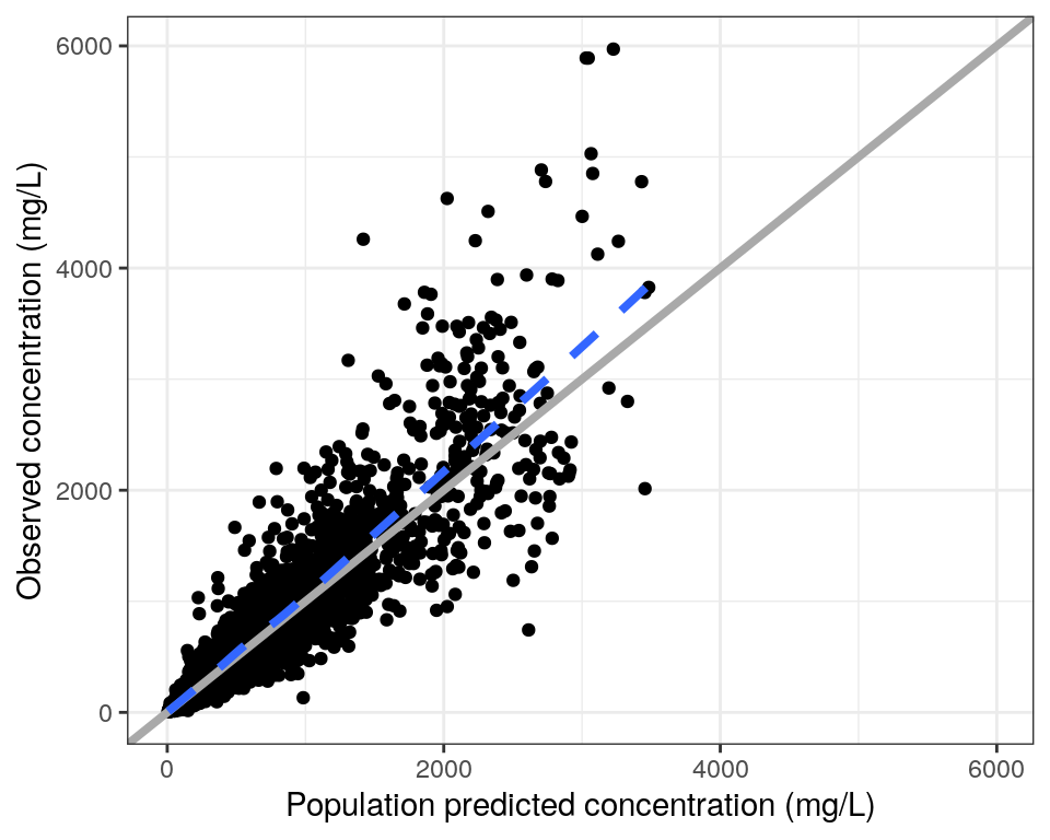
dvip <- dv_ipred(data, yname = "concentration (mg/L)")
dvip <- dv_ipred(
  data,
  yname = "concentration (mg/L)"
)
dvip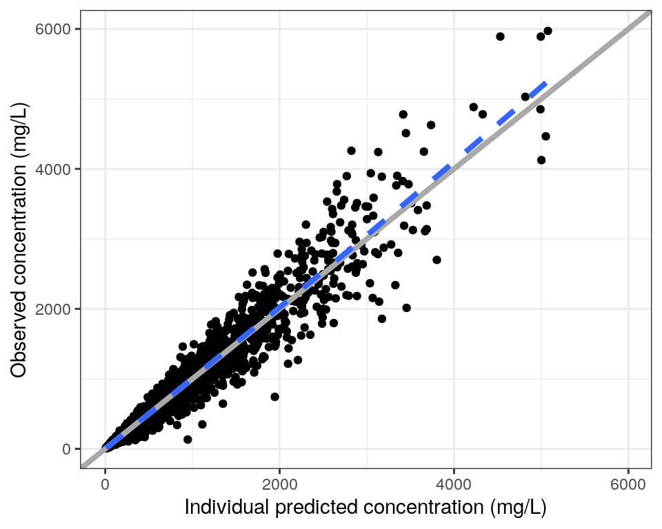
As these predictions are based on samples from the posterior, we also have access to upper and lower percentiles of EPRED, IPRED, NPDE, and EWRES in the columns with the _lo and _hi suffixes. By default, these represent the 2.5th and 97.5th percentiles, but other percentiles can be requested in the probs argument of nm_join_bayes. We can represent the uncertainty in model predictions using these percentiles to plot credible intervals. For example, the custom code below plots DV vs EPRED with credible intervals.
dvp_ci <- ggplot(data = data, aes(x = EPRED, y = DV)) +
  geom_errorbarh(aes(xmin = EPRED_lo, xmax = EPRED_hi),
                 colour = "red3", alpha = 0.3) +
  geom_point() +
  xlab(glue("Population predicted concentration (mg/L)")) +
  ylab("Observed concentration (mg/L)") +
  pm_abline() +
  pm_smooth() +
  pm_theme()
dvp_ci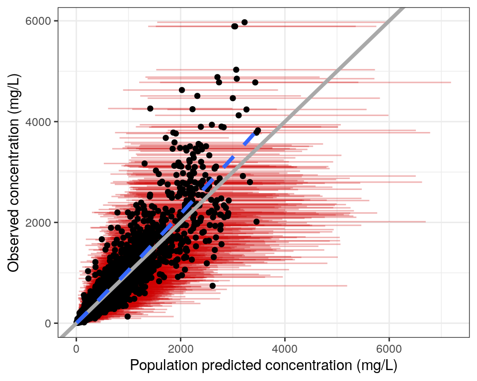
Individual observed vs predicted plots
Individual plots of DV, EPRED, and IPRED vs time (linear and log scale) are generated with the dv_pred_ipred function. These plots are highly customizable, but we show the first plot from a simple example here:
dvip <- dv_pred_ipred(
  data,
  pred = "EPRED//Population predicted concentration (mg/L)",
  id_per_plot = 9,
  ncol = 3,
  angle = 45,
  use_theme = theme_bw()
)
dvip[[1]]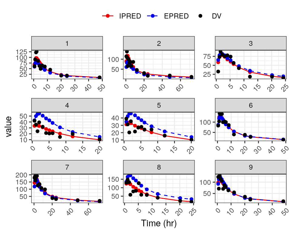
NPDE Plots
The pmplots package includes a series of functions for plotting normalized prediction distribution errors (NPDEs):
npde_predNPDE vs the population predictions (PRED by default, but we use EPRED here)npde_timeNPDE vs timenpde_tadNPDE vs time after dose (TAD)npde_contNPDE vs continuous covariatesnpde_catNPDE vs categorical covariatesnpde_histdistribution of NPDEsnpde_qquantile-quantile of NPDEs
Again, these functions can be customized. Below, we show how to swap PRED to EPRED, customize the axis labels using information in your spec file, map across multiple covariates, and panel multiple plots into a single figure with the pm_grid function or the patchwork package.
These applications of the pmplots NPDE functions are almost identical to those in the Expo 1 Model Diagnostics. The only exception being that we use EPRED instead of PRED for population predictions.
NPDE vs population predictions, time, and time after dose
The pmplots package provides basic, intuitive axes labels automatically for plots created using its functions. However, it also includes a series of functions to customize those labels. Here, we demonstrate how to grab the units for time from your spec object, append them to the time labels, and how to include your models specific endpoint with units (in this case, concentration (mg/L)).
xTIME <- pm_axis_time(spec$TIME$unit)
xTIME
[1] "TIME//Time (h)"xTAD <- pm_axis_tad(spec$TAD$unit)
xPRED <- "EPRED//Population predicted concentration (mg/L)"p1 <- npde_pred(data, x = xPRED, y = "NPDE // ")
p2 <- npde_time(data, x = xTIME)
p3 <- npde_tad(data, x = xTAD, y = "NPDE // ")
p <- p1 / p2 / p3
p 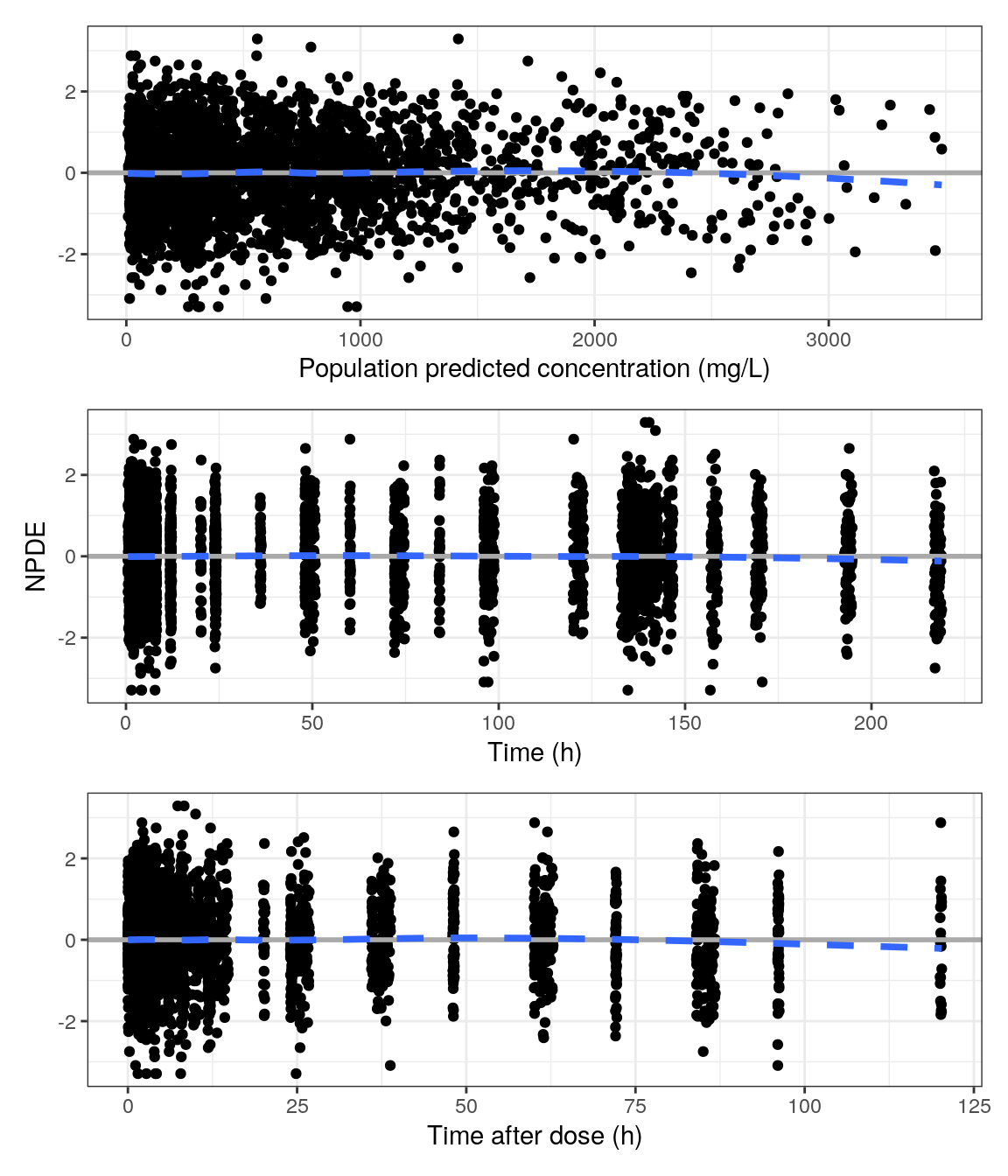
NPDE vs continuous covariates
The NPDE vs continuous covariate plots leverage the information in your spec object in two main ways:
- the covariates of interest are extracted from the covariate flags in your spec file using the
pull_metafunction fromyspec(also described above). - the axis labels are renamed with the short label in the spec
diagContCov <- pull_meta(spec, "flags")$diagContCov

NPDEco <- spec %>%
  ys_select(all_of(diagContCov)) %>%
  axis_col_labs(title_case = TRUE, short_max = 10) %>%
  as.list()

NPDEco
$AGE
[1] "AGE//Age (years)"
$WT
[1] "WT//Weight (kg)"
$ALB
[1] "ALB//Albumin (g/dL)"
$EGFR
[1] "EGFR//EGFR (mL/min/1.73m2)"pList <- purrr::map(NPDEco, ~ npde_cont(data, x = .x))
pm_grid(pList, ncol = 2)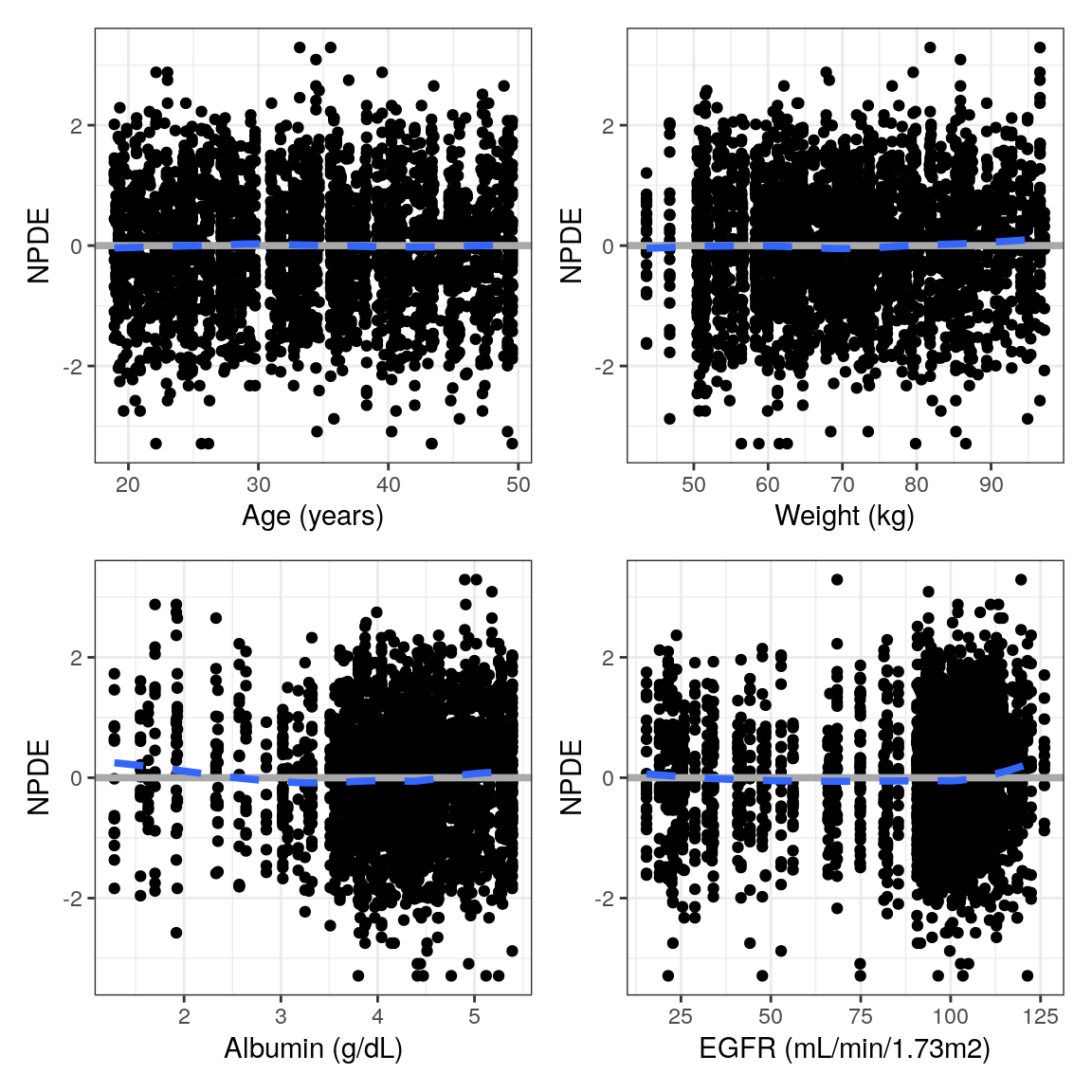
NPDE vs categorical covariates
The information in the spec object was used to to rename the axis labels. These plots also used the spec object to decode the numerical categorical covariate categories (shown above).
NPDEca <- spec %>%
  ys_select("RF", "CP") %>%
  axis_col_labs(title_case = TRUE, short_max = 20) %>%
  as.list()
pList_cat <- purrr::map(NPDEca, ~ npde_cat(data, x = .x))
pm_grid(pList_cat, ncol=1)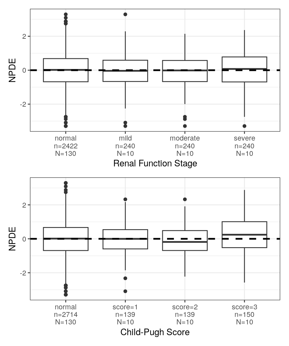
NPDE histogram
Here, we show an NPDE density plot, but the y-axis can be customized to show count or density.
p <- npde_hist(data)
p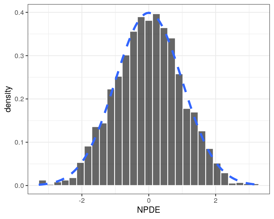
Other residual plots
The pmplots package includes a similar series of functions to create other residual plots. They’re all similarly named but, instead of beginning with npde_, they’re prefaced with:
res_for residual functions/plotswres_for weighted residual functions/plotscwres_for conditional weighted residual functions/plotscwresi_for conditional weighted residual with interaction functions/plots
We want to plot the simulation-based EWRES instead of CWRES, so we use the res_ plots and specify the appropriate column and label.
yEWRES <- "EWRES//Expected weighted residual"Below are a couple of examples of EWRES plots.
EWRES vs population predictions, time and time after dose
p1 <- res_pred(data, x = xPRED, y = "EWRES //  ")
p2 <- res_time(data, x = xTIME, y = yEWRES)
p3 <- res_tad(data, x = xTAD, y = "EWRES //  ")
p <- p1 / p2 / p3
p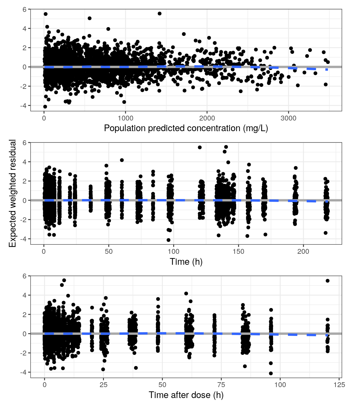
EWRES quantile-quantile (QQ) and density histogram
p <- wres_q(data, x = "EWRES") / res_hist(data, x = yEWRES)
p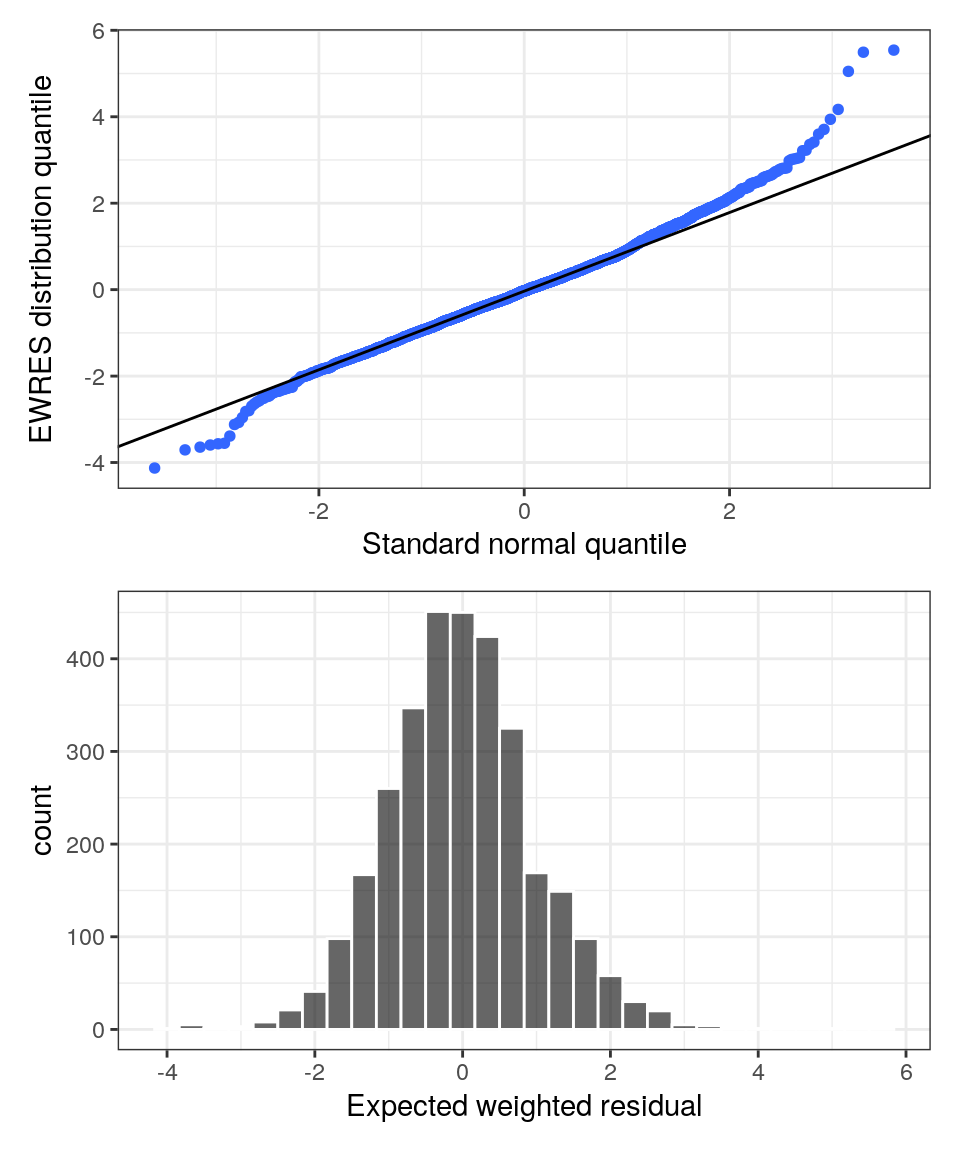
EBE-based diagnostics
Again, these diagnostics are almost identical in process to those in the Expo 1 Model Diagnostics. The only exception being that the ETAs are now generated by summarizing over the full posterior (if .iph files are available).
The ETA based plots require a dataset filtered to one record per subject.
id <- distinct(data, ID, .keep_all=TRUE) Here we show how to plot:
eta_pairsthe correlation and distribution of model ETAseta_contETA vs continuous covariateseta_catETA vs categorical covariates
Again we’ll leverage the information in the spec object in several ways:
- the covariates of interest are extracted from the covariate flags in your spec file using the
pull_metafunction, and those covariates are selected from the spec object usingys_selectfunction (also described above) - the axis labels are renamed with the short label in the spec using
axis_col_labs - numerical categorical covariates are decoded with the
yspec_add_factorsfunction
The ETAs to be plotted can either be extracted programatically,
etas <- stringr::str_subset(names(data), "ETA")or you can create a list with labels that replace the ETA numbers in your plots.
etas <- c("ETA1//ETA-KA", "ETA2//ETA-V/F", "ETA3//ETA-CL/F")ETA pairs plot
p <- eta_pairs(id, etas)
p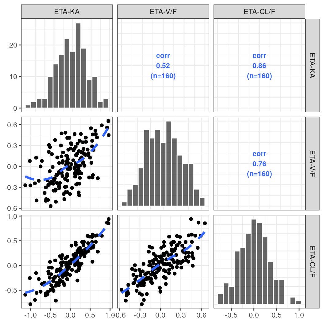
ETA vs continuous covariates
Here, we use a map_wrap_eta_cont function to generate plots of all continuous covariates vs each ETA value in a single line. Note that, in this case, we map over the ETAs and produce one plot per ETA faceted by continuous covariates. Below, we show a similar example for categorical covariates, but we’ll create one plot per covariate and ETA pair. For brevity, we’ll show an example of the first plot, but the code produces one plot per ETA.
co <- spec %>%
  ys_select(all_of(diagContCov)) %>%
  axis_col_labs(title_case = TRUE, short_max = 10)

p <- purrr::map(.x = etas, ~ map_wrap_eta_cont(.x, co, id))
p[[1]]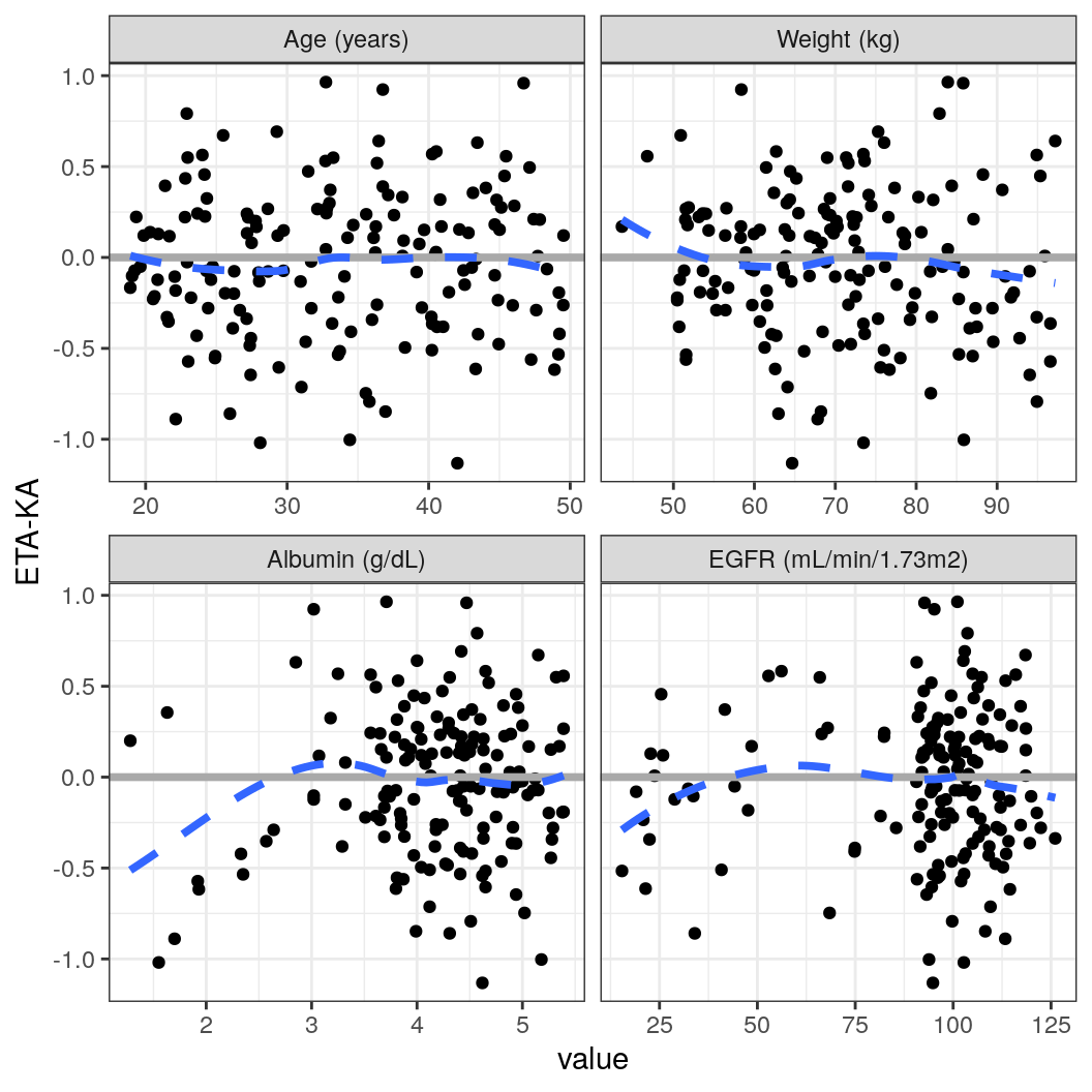
ETA vs categorical covariate
Here, we show how to map over the categorical covariates of interest and to create one plot per covariate and ETA pair. These plots can be combined using the patchwork package.
ca <- spec %>%
  ys_select(all_of(diagCatCov)) %>%
  axis_col_labs(title_case=TRUE, short_max = 20)
p <- eta_cat(id, ca, etas)
pRenal <- (p[[5]] + p[[6]]) / (p[[7]] + p[[8]])
pRenal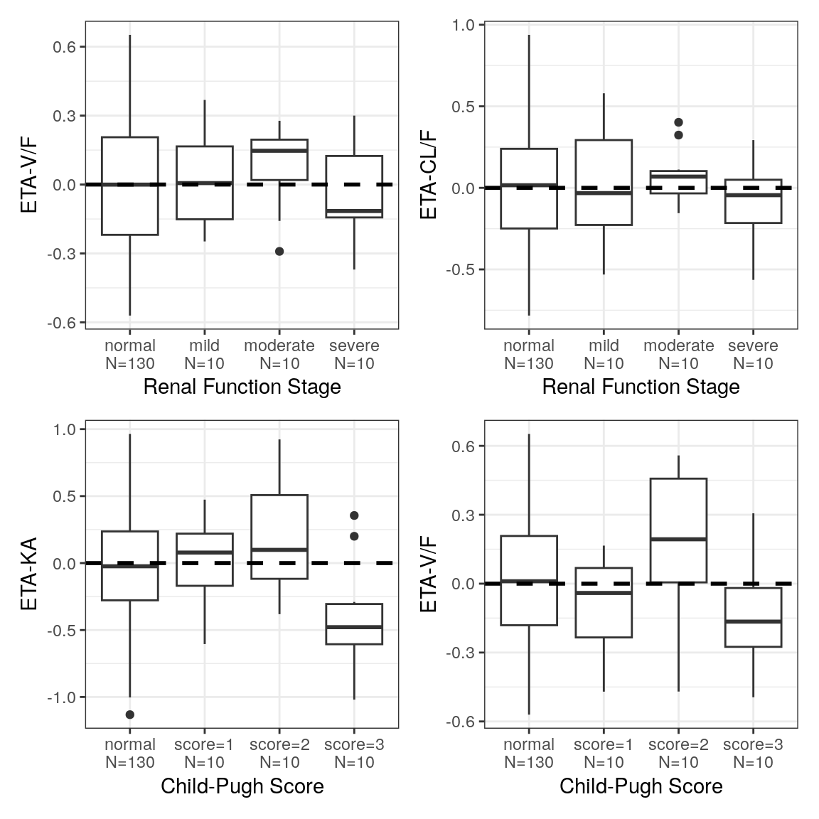
Other resources
The scripts discussed on this page can be found in the GitHub repository. To run this code you should consider visiting the About the GitHub Repo page first.
Diagnostic templates
- Code shown on this page is available:
template-model-bayes.Rmd.
Diagnostic scripts
- The functions (not in packages) used in these diagnostics is available here: functions-diagnostics.R.
- The code to render these model diagnostics as a parameterized report is available: model-diagnostics.R.
Publications
- Johnston CK, Waterhouse T, Wiens M, Mondick J, French J, Gillespie WR. Bayesian estimation in NONMEM. CPT Pharmacometrics Syst Pharmacol. 2023; 00: 1-16. doi.org/10.1002/psp4.13088
- Nguyen et al. Model Evaluation of Continuous Data Pharmacometric Models: Metrics and Graphics. CPT Pharmacometrics Syst Pharmacol. 2017 Feb;6(2):87-109.
- Byon et al. Establishing best practices and guidance in population modeling: an experience with an internal population pharmacokinetic analysis guidance. CPT Pharmacometrics Syst Pharmacol. 2013 Jul 3;2(7):e51. doi: 10.1038/psp.2013.26. PMID: 23836283; PMCID: PMC6483270.