library(tidyverse)
theme_set(theme_bw())
library(yspec)
library(mrgsolve)
library(mrggsave)
library(vpc)
library(glue)
library(bbr)
library(bbr.bayes)
library(here)
library(posterior)Introduction
This document illustrates the mechanics of using the vpc package along with mrgsolve to create visual predictive check (VPC) plots for NONMEM® Bayesian (Bayes) models.
Tools used
MetrumRG packages
mrgsolve Simulate from ODE-based population PK/PD and QSP models in R.
yspec Data specification, wrangling, and documentation for pharmacometrics.
bbr Manage, track, and report modeling activities, through simple R objects, with a user-friendly interface between R and NONMEM®.
bbr.bayes Extension of the bbr package to support Bayesian modeling with Stan or NONMEM®.
mrggsave Label, arrange, and save annotated plots and figures.
CRAN packages
Outline
- Load the analysis data set used during the NONMEM® model estimation
- Load an
mrgsolvetranslation of the NONMEM® model and validate the coding against outputs from the NONMEM® run - Simulate data replicates from the
mrgsolvemodel - Construct four VPCs:
- Basic VPC of dose-normalized concentrations
- VPC for a single dose, stratified by a covariate
- VPC of the fraction below the quantitative limit versus time
- Prediction-corrected VPC
Differences for Bayes models
This process largely follows the steps outlined for maximum likelihood NONMEM® models in Visual predictive check from Expo 1 with the following differences:
- As with VPCs for maximum likelihood models, parameter uncertainty was not included in simulations. VPCs for a Bayes model used the median of the posterior instead of the parameter estimates directly from NONMEM® output
- For mrgsolve model validation, output from the first chain is used to exactly match PRED and IPRED from NONMEM®
- For prediction-corrected VPCs, Bayes models use EPRED from
nm_join_bayesinstead of PRED
Required packages
All packages were installed from MPN via pkgr.
These are some global options reflecting the directory structure associated with this project
options(mrggsave.dir = tempdir(), mrg.script = "pk-vpc-final.Rmd")
options(mrgsolve.project = here("script/model"))
This is a theme that we use to style the plots coming out of vpc
mrg_vpc_theme = new_vpc_theme(list(
  sim_pi_fill = "steelblue3", sim_pi_alpha = 0.5,
  sim_median_fill = "grey60", sim_median_alpha = 0.5
))
Setup
Data
First, we have some observations that are below the limit of quantification (BLQ) that need to be dealt with.
The final model estimation run was 1100, so we read in the dataset used for that model with bbr::nm_data(). You can read more about using bbr and bbr.bayes for model management in Model Management.
runno <- 1100
MODEL_DIR <- here("model/pk")
mod_bbr <- read_model(file.path(MODEL_DIR, runno))
data <- nm_data(mod_bbr)
We load in the complete data including observations that were ignored in the estimation run; because, they were below the BLQ and exclude only commented records
data <- filter(data, is.na(C))

head(data)
# A tibble: 6 × 34
C NUM ID TIME SEQ CMT EVID AMT DV AGE WT HT EGFR
<lgl> <int> <int> <dbl> <int> <int> <int> <int> <dbl> <dbl> <dbl> <dbl> <dbl>
1 NA 1 1 0 0 1 1 5 0 28.0 55.2 160. 114.
2 NA 2 1 0.61 1 2 0 NA 61.0 28.0 55.2 160. 114.
3 NA 3 1 1.15 1 2 0 NA 91.0 28.0 55.2 160. 114.
4 NA 4 1 1.73 1 2 0 NA 122. 28.0 55.2 160. 114.
5 NA 5 1 2.15 1 2 0 NA 126. 28.0 55.2 160. 114.
6 NA 6 1 3.19 1 2 0 NA 84.7 28.0 55.2 160. 114.
# ℹ 21 more variables: ALB <dbl>, BMI <dbl>, SEX <int>, AAG <dbl>, SCR <dbl>,
# AST <dbl>, ALT <dbl>, CP <int>, TAFD <dbl>, TAD <dbl>, LDOS <int>,
# MDV <int>, BLQ <int>, PHASE <int>, STUDYN <int>, DOSE <int>, SUBJ <int>,
# USUBJID <chr>, STUDY <chr>, ACTARM <chr>, RF <chr>We use the data specification object that corresponds with the model estimation data (in this case pk)
spec <- ys_load(here("data/derived/pk.yml"))
spec <- ys_namespace(spec, "long")
The ys_get_short_unit() function pulls the “short” name from each column name and appends the unit if available
lab <- ys_get_short_unit(spec, parens = TRUE, title_case = TRUE)The ys_add_factors() function looks at spec for discrete data items and appends them to the data set as factors
data <- ys_add_factors(data, spec)For example:
count(data, CP, CP_f)# A tibble: 4 × 3
CP CP_f n
<int> <fct> <int>
1 0 CP score: 0 3880
2 1 CP score: 1 160
3 2 CP score: 2 160
4 3 CP score: 3 160For convenience, we set aliases for a couple of these columns
data <- mutate(data, Hepatic = CP_f, Renal = RF_f)The simulation model
Read in the mrgsolve model corresponding to the NONMEM® model model/pk/1100.ctl
mod0 <- mread(glue("{runno}.mod"))Setting parameter values for simluation model
The mrgsolve model uses an nmext block as a convenience to set up the THETAs, OMEGAs, and SIGMAs correctly. However, this requires reading in values from an .ext file so the following is set up to read in from the first chain (1100-1) only:
[ nmext ]
path = '../../model/pk/1100/1100-1/1100-1.ext'
root = 'cppfile'
These estimates (means of the first chain posterior) need to be overwritten with the medians of the full posterior (across all chains).
First, extract the posterior draws
draws <- read_fit_model(mod_bbr)Then, calculate the posterior median for each parameter and separate into THETAs, OMEGAs, and SIGMAs, constructing matrices for OMEGAs and SIGMAs. Depending on your mrgsolve model, this may need some tweaking for different block structures for OMEGA or SIGMA
params <- draws %>%
  subset_draws(variable = c("THETA", "OMEGA", "SIGMA")) %>%
  summarize_draws(median) %>%
  mutate(variable = str_remove_all(variable, "[:punct:]")) %>%
  pivot_wider(names_from = variable, values_from = median)
theta <- params %>% select(starts_with("THETA"))
omega <- params %>%
  select(starts_with("OMEGA")) %>%
  bmat()
sigma <- params %>%
  select(starts_with("SIGMA")) %>%
  bmat()
Finally, update the mrgsolve model to use these posterior medians
mod <- mod0 %>%
  param(theta) %>%
  omat(omega) %>%
  smat(sigma)
Validate simulation model
We can validate our mrgsolve model code by looking at the PRED and IPRED values returned from NONMEM® as compared to PRED and IPRED returned from the mrgsolve model simulation. For this we revert to the mod0 object, which uses estimates from the first NONMEM® chain. This allows us to easily generate PRED and IPRED values associated with the first chain by setting ETAs to zero (for PRED) or the post hoc values reported by NONMEM® (for IPRED).
PRED and IPRED are extracted from the first chain output using nm_join.
mod_chn1 <- read_model(file.path(MODEL_DIR, runno, glue("{runno}-1")))
data_chn1 <- nm_join(mod_chn1)
select(data_chn1, ID, TIME, DV, IPRED, PRED)
# A tibble: 4,292 × 5
ID TIME DV IPRED PRED
<int> <dbl> <dbl> <dbl> <dbl>
1 1 0 0 0 0
2 1 0.61 61.0 69.1 62.8
3 1 1.15 91.0 91.3 80.6
4 1 1.73 122. 97.6 84.7
5 1 2.15 126. 97.0 83.5
6 1 3.19 84.7 89.0 76.3
7 1 4.21 62.1 79.2 68.4
8 1 5.09 49.1 71.5 62.1
9 1 6.22 64.2 62.8 55.1
10 1 8.09 59.6 51.4 45.8
# ℹ 4,282 more rowsFirst we validate PRED by simulating it from the NONMEM® output with the IIV zeroed out. We modify the mrgsolve model object to return PRED when we simulate
check_pred <- mod0 %>%
  zero_re() %>%
  mrgsim(data = data_chn1, recover = "PRED,EVID", digits = 5)

head(check_pred) %>% select(ID, TIME, Y, PRED)
ID TIME Y PRED
1 1 0.00 0.000 0.000
2 1 0.61 62.793 62.793
3 1 1.15 80.647 80.647
4 1 1.73 84.669 84.669
5 1 2.15 83.544 83.544
6 1 3.19 76.311 76.311Keeping only observations
check_pred <- filter(check_pred, EVID == 0)We do a quick summary and show that all 3142 PRED values match between the mrgsolve model and NONMEM® output
nrow(check_pred) [1] 3142summary(check_pred$Y - check_pred$PRED) Min. 1st Qu. Median Mean 3rd Qu. Max.
-0.1000000 0.0000000 0.0000000 -0.0005485 0.0000000 0.1000000 Next we validate with IPRED, with the IIV coming from the post hoc ETAs in the dataset, using the etasrc argument in mrgsim. Otherwise, the process is similar to what we did for PRED
check_pred <- mod0 %>%
  zero_re() %>%
  mrgsim(data = data_chn1, recover = "IPRED,EVID", digits = 5,
         etasrc = "data.all")

check_pred <- filter(check_pred, EVID == 0)
summary(check_pred$Y - check_pred$IPRED)
Min. 1st Qu. Median Mean 3rd Qu. Max.
0 0 0 0 0 0 This demonstrates that the simulation model can reproduce the population and individual predictions from the estimation model and is reliable for use to simulate the predictive check.
VPC on dose-normalized concentrations
In this example, we normalize the observed and simulated data from single-ascending dose (SAD) and multiple-ascending dose (MAD) studies (Studies 1 and 2) and present all doses in the same plot.
Studies 1 and 2 included healthy volunteers.
count(data, STUDY, STUDYN, CP_f, RF_f)# A tibble: 10 × 5
STUDY STUDYN CP_f RF_f n
<chr> <int> <fct> <fct> <int>
1 101-DEMO-001 1 CP score: 0 No impairment 480
2 101-DEMO-002 2 CP score: 0 No impairment 1800
3 201-DEMO-003 3 CP score: 0 No impairment 360
4 201-DEMO-003 3 CP score: 0 Mild impairment 360
5 201-DEMO-003 3 CP score: 0 Moderate impairment 360
6 201-DEMO-003 3 CP score: 0 Severe impairment 360
7 201-DEMO-004 4 CP score: 0 No impairment 160
8 201-DEMO-004 4 CP score: 1 No impairment 160
9 201-DEMO-004 4 CP score: 2 No impairment 160
10 201-DEMO-004 4 CP score: 3 No impairment 160sad_mad <- filter(data, STUDYN <= 2)The simulation function
We create a function to simulate out one replicate and re-use it for all the different simulations performed for the predictive checks.
sim <- function(rep, data, model,
                recover = "EVID,DOSE,STUDY,Renal,Hepatic") {
  mrgsim(
    model,
    data = data,
    carry_out = "NUM",
    recover = recover,
    Req = "Y",
    output = "df"
  ) %>%  mutate(irep = rep)
}
Arguments
repthe current replicate numberdatathe data template for simulationmodelthe mrgsolve model objectrecovercolumns to carry from the data into the output
Return
A data frame with the replicate number appended as irep.
Simulate for VPC
We simulate only 100 replicates here to save some computation time; we would typically simulate more in a production context.
isim <- seq(100)

set.seed(86486)

sims <- lapply(
  isim, sim,
  data = sad_mad,
  mod = mod
) %>% bind_rows()
Filter both the observed and simulated data on
- actual observations that are not BLQ
- simulated observations that are above the limit of quantification (here 10 ng/mL)
fsad_mad <-  filter(sad_mad,  EVID == 0, BLQ == 0)
fsims <- filter(sims, EVID == 0, Y >= 10)
Also, we dose-normalize the observed and simulated data so all doses can be combined on the same plot
fsad_mad <-  mutate(fsad_mad,  DVN = DV/DOSE)
fsims <- mutate(fsims, YN = Y/DOSE)
Calculate VPC and plot
Pass observed and simulated data into the vpc() function, noting that we want this stratified by STUDY so that SAD and MAD regimens are plotted separately
p1 <- vpc(
  obs = fsad_mad,
  sim = fsims,
  stratify = "STUDY",
  obs_cols = list(dv = "DVN"),
  sim_cols = list(dv = "YN", sim = "irep"),
  log_y = TRUE,
  pi = c(0.05, 0.95),
  ci = c(0.025, 0.975),
  facet = "columns",
  show = list(obs_dv = TRUE),
  vpc_theme = mrg_vpc_theme
)
Notes
- This VPC should show dose-normalized concentrations, so we change the name of
dvunderobs_colsandsim_cols - Setting
pitoc(0.05, 0.95)indicates that the VPC displays the 5th and 95th percentiles of observed and simulated data in addition to the median - Setting
citoc(0.025, 0.975)indicates that the VPC displays the 95% prediction intervals around the simulated statistics (median, 5th and 95th percentiles - The
showargument indicates that observed data points should be included on the plot
p1 <-
  p1 +
  xlab(lab$TIME) +
  ylab("Dose-normalized concentration (ng/mL)")

p1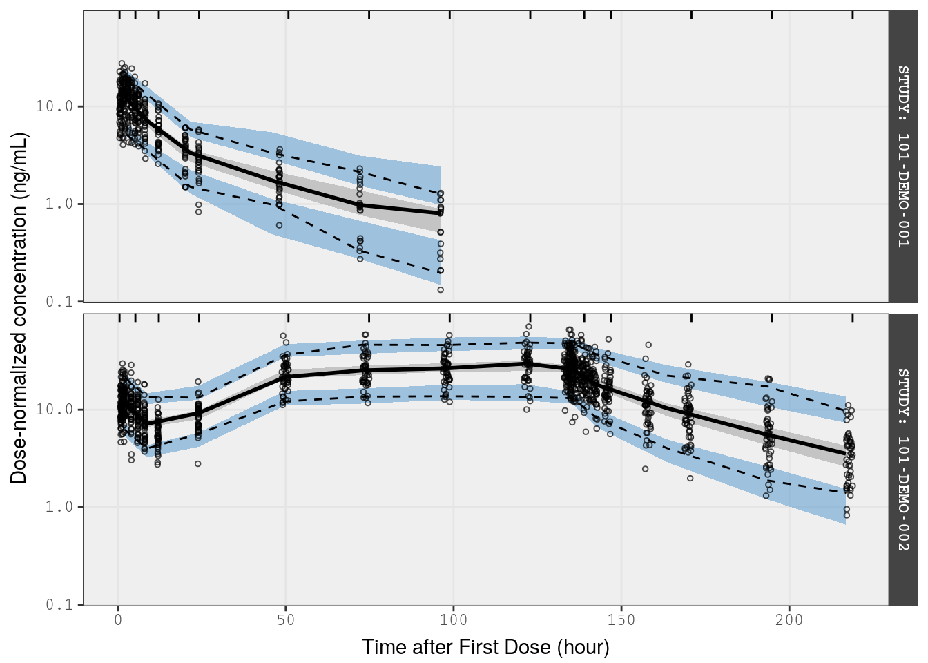
mrggsave_last(stem = "pk-vpc-{runno}-dose-norm", height = 7.5)VPC stratified on a covariate
In this example, we take a subset of the data from the renal study (Study 3) and stratify the VPC on the renal function covariate
rf_data <- filter(data, STUDYN == 3) set.seed(54321)
rf_sims <- lapply(
isim, sim,
data = rf_data,
mod = mod
) %>% bind_rows()Filtering both the observed and simulated data, there was only a single dose administered in this study
f_rf_data <- filter(rf_data, EVID == 0, BLQ == 0)
f_rf_sims <- filter(rf_sims, EVID == 0, Y >= 10)
Run the vpc function and plot
p2 <- vpc(
  obs = f_rf_data,
  sim = f_rf_sims,
  stratify = "Renal",
  obs_cols = list(dv = "DV"),
  sim_cols = list(dv = "Y", sim = "irep"),
  log_y = TRUE,
  pi = c(0.05, 0.95),
  ci = c(0.025, 0.975),
  show = list(obs_dv = TRUE),
  vpc_theme = mrg_vpc_theme
)

p2 <- p2 +  xlab(lab$TIME) + ylab("Concentration (ng/mL)")

p2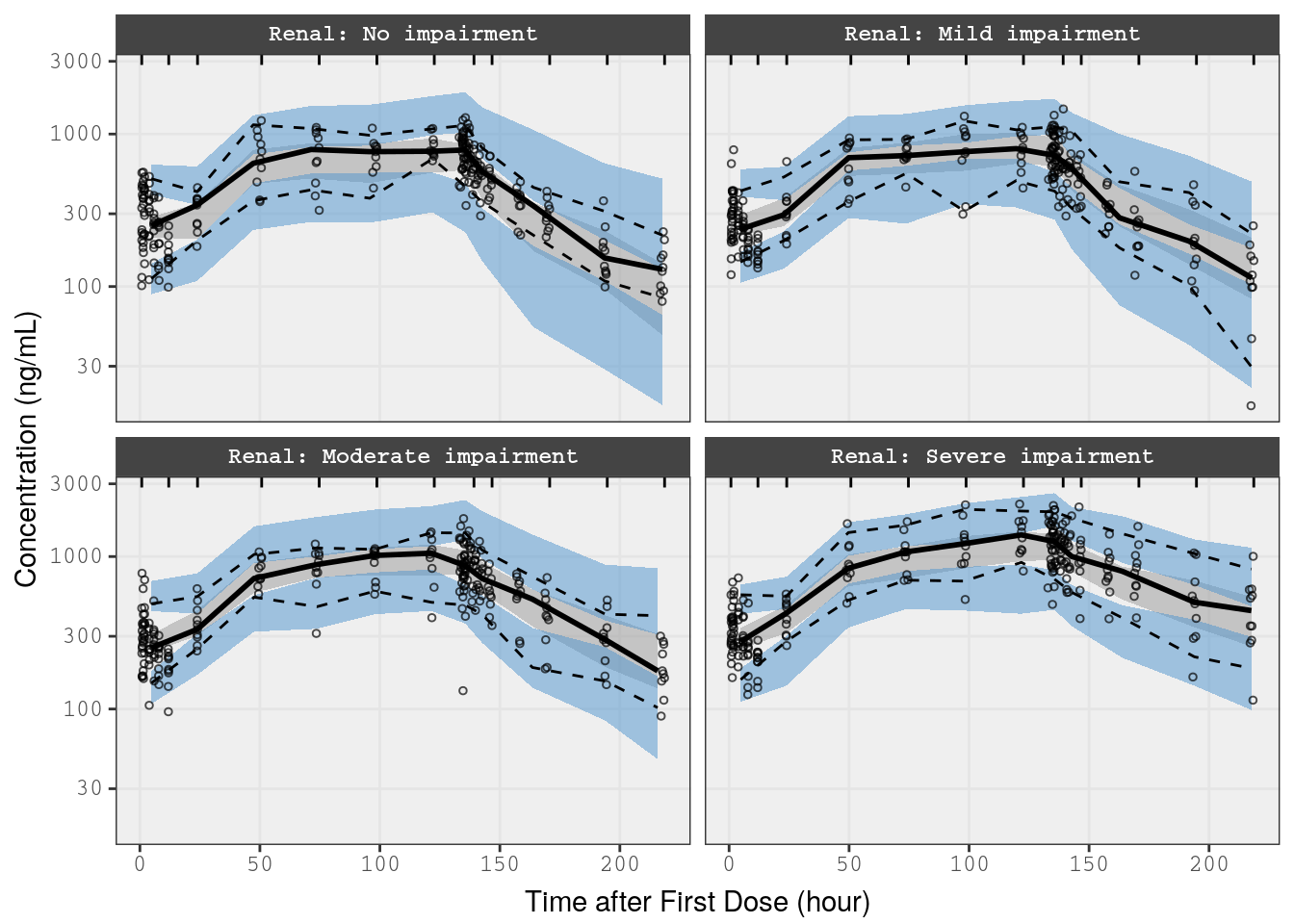
mrggsave_last(stem = "pk-vpc-{runno}-rf", height = 6.5)Alternatively, run the vpc function stratified on hepatic function
Show the code
cp_data <- filter(data, STUDYN==4)

set.seed(7456874)

cp_sims <- lapply(
  isim,
  sim,
  data = cp_data,
  mod = mod
) %>% bind_rows()

f_cp_data <- filter(cp_data, EVID==0, BLQ ==0)
f_cp_sims <- filter(cp_sims, EVID==0, Y >= 10)

p3 <- vpc(
  obs = f_cp_data,
  sim = f_cp_sims,
  stratify = "Hepatic",
  obs_cols = list(dv = "DV"),
  sim_cols=list(dv="Y", sim="irep"),
  log_y = TRUE,
  pi = c(0.05, 0.95),
  ci = c(0.025, 0.975),
  labeller = label_value,
  show = list(obs_dv = TRUE),
  vpc_theme = mrg_vpc_theme
)

p3 <-
  p3 +
  xlab(lab$TIME) +
  ylab("Concentration (ng/mL)")

p3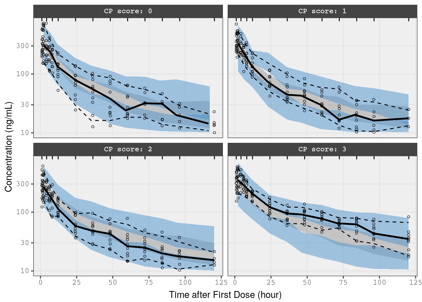
mrggsave(p3, stem = "pk-vpc-{runno}-cp", height = 6.5)VPC on fraction BLQ
This is a predictive check of the fraction of observations that are BLQ versus time. We take just the single dose studies and limit the analysis out to 100 hours after the dose
data_fracblq <- filter(data, STUDYN %in% c(1, 3), TIME <= 100)Simulate using the sim() function as we have done before
set.seed(7456874)

b_sims <- lapply(
  isim,
  sim,
  data = data_fracblq,
  mod = mod
) %>% bind_rows()
Now, we use the vpc_cens() function from the vpc package and pass in the lower limit of quantification (lloq)
p4 <- vpc_cens(
  sim = b_sims,
  obs = data_fracblq,
  lloq = 10,
  obs_cols = list(dv = "DV"),
  sim_cols = list(dv = "Y", sim = "irep")
)

p4 <- p4 + xlab(lab$TIME)

p4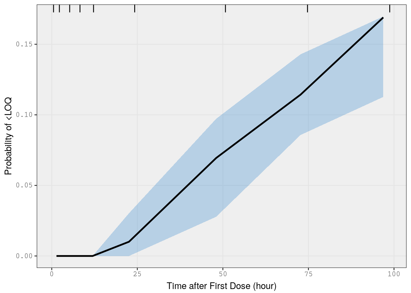
mrggsave_last(stem = "pk-vpc-{runno}-BLQ", height = 6.5)Prediction-corrected VPC
This VPC method removes variability in a time bin by “correcting” (or normalizing) observed and simulated data with the population predicted value. For the population predictions, we use EPRED generated by nm_join_bayes. For more details on the nm_join_bayes function, see the Model Diagnostics page.
We load in the complete data, including observations that were ignored in the estimation run because they were BLQ. To do this, pass .superset = TRUE to nm_join_bayes. The result is the full model estimation data set along with all items that were tabled from that run. Be sure to drop any rows that were excluded from the model estimation run for reasons other than being BLQ before proceeding.
As we only need EPRED (and the original data) we can skip IPRED, EWRES, and NPDE.
set.seed(1)
progressr::with_progress({
  data0 <- mod_bbr %>%
    nm_join_bayes(
      mod_mrgsolve = mod,
      .superset = TRUE,
      ipred = FALSE,
      ewres_npde = FALSE
    )
})
data <- filter(data0, is.na(C))
This dataset now includes EPRED, but we don’t have those values for rows where the observations were BLQ. We use mrgsolve to simulate EPRED for every row in the complete data set, approximated by predictions with all variability set to zero.
out <- mrgsim(zero_re(mod), data)Then, we copy that value into the simulation data set for use in the prediction-corrected VPC
data <- mutate(data, EPRED = ifelse(BLQ > 0, out$Y, EPRED))Taking just single dose studies (1 and 4)
single <- filter(data, STUDYN %in% c(1,4))out <- lapply(
seq(200),
FUN = sim,
data = single,
model = mod,
recover = "EPRED,DV,EVID,DOSE"
) %>% bind_rows()Get simulated and observed data ready so that EPRED is in both the simulated and observed data
observed <- filter(single, EVID == 0, BLQ == 0)
simulated <- filter(out,   EVID == 0, Y >= 10)

head(simulated)
ID TIME NUM Y EPRED DV EVID DOSE irep
1 1 0.61 2 48.72265 58.56252 61.005 0 5 1
2 1 1.15 3 77.11560 75.01682 90.976 0 5 1
3 1 1.73 4 132.37288 77.65459 122.210 0 5 1
4 1 2.15 5 106.34826 78.89718 126.090 0 5 1
5 1 3.19 6 74.47268 72.93105 84.682 0 5 1
6 1 4.21 7 95.51301 65.92059 62.131 0 5 1head(observed)# A tibble: 6 × 54
C NUM ID TIME SEQ CMT EVID AMT DV.DATA AGE WT HT
<lgl> <dbl> <int> <dbl> <int> <int> <int> <int> <dbl> <dbl> <dbl> <dbl>
1 NA 2 1 0.61 1 2 0 NA 61.0 28.0 55.2 160.
2 NA 3 1 1.15 1 2 0 NA 91.0 28.0 55.2 160.
3 NA 4 1 1.73 1 2 0 NA 122. 28.0 55.2 160.
4 NA 5 1 2.15 1 2 0 NA 126. 28.0 55.2 160.
5 NA 6 1 3.19 1 2 0 NA 84.7 28.0 55.2 160.
6 NA 7 1 4.21 1 2 0 NA 62.1 28.0 55.2 160.
# ℹ 42 more variables: EGFR <dbl>, ALB <dbl>, BMI <dbl>, SEX <int>, AAG <dbl>,
# SCR <dbl>, AST <dbl>, ALT <dbl>, CP <int>, TAFD <dbl>, TAD <dbl>,
# LDOS <int>, MDV <int>, BLQ <int>, PHASE <int>, STUDYN <int>, DOSE <int>,
# SUBJ <int>, USUBJID <chr>, STUDY <chr>, ACTARM <chr>, RF <chr>, CL <dbl>,
# V2 <dbl>, Q <dbl>, V3 <dbl>, KA <dbl>, ETA1 <dbl>, ETA2 <dbl>, ETA3 <dbl>,
# ETA4 <dbl>, ETA5 <dbl>, IPRED <dbl>, NPDE <dbl>, EWRES <dbl>, DV <dbl>,
# PRED <dbl>, RES <dbl>, WRES <dbl>, EPRED <dbl>, EPRED_lo <dbl>, …Now in the vpc function call, we can set pred_corr = TRUE. We also need to specify pred = "EPRED" as the default column is PRED.
p5 <- vpc(
  obs = observed,
  sim = simulated,
  obs_cols = list(dv = "DV", pred = "EPRED"),
  sim_cols = list(dv = "Y", sim = "irep", pred = "EPRED"),
  log_y = TRUE,
  pred_corr = TRUE,
  pi = c(0.05, 0.95),
  ci = c(0.025, 0.975),
  labeller = label_value,
  show = list(obs_dv = TRUE),
  vpc_theme = mrg_vpc_theme
)
p5 <-
p5 +
xlab(lab$TIME) +
ylab("Pred-corrected concentration (ng/mL)")
p5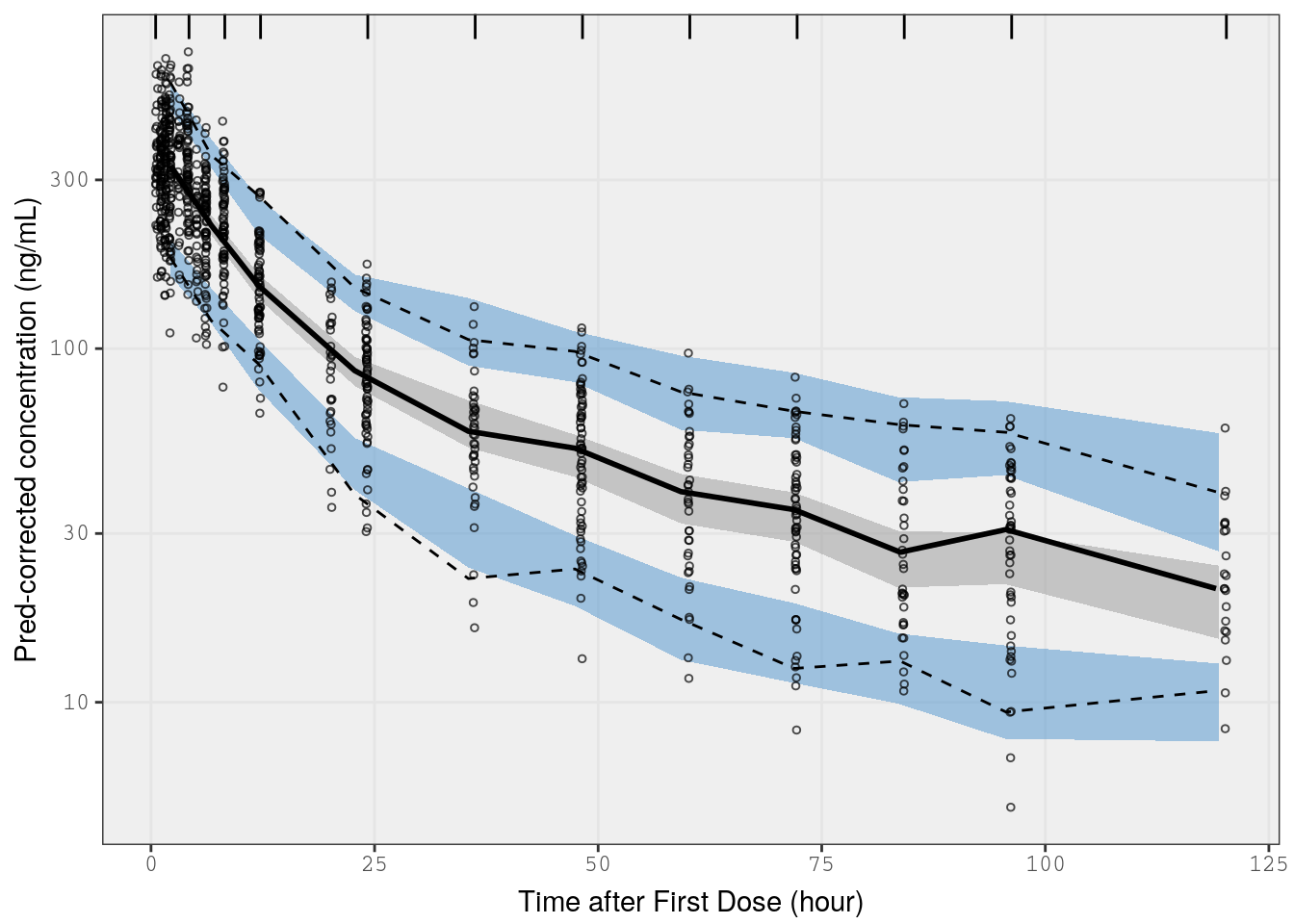
mrggsave_last(stem = "pk-vpc-{runno}-pc", height = 6.5)Other resources
The following scripts from the GitHub repository are discussed on this page. If you’re interested running this code, visit the About the GitHub Repo page first.
PK VPC script: pk-vpc-final.R
PK PCVPC script: pk-pcvpc-final.R