library(tidyverse)
library(pmtables)
library(here)
library(bbr)
library(bbr.bayes)
library(magrittr)
library(yaml)
library(posterior)Introduction
Generating clear, well-formatted parameter tables for your NONMEM® model is an important part of reporting your model results, but it is often a tedious, time-consuming process. Here, we show how to quickly and simply create parameter tables by leveraging a few intuitive functions designed to:
- Read in your model parameters from various NONMEM® output files
- Describe your model parameters in a
.YAMLfile - Back-transform any parameters estimated in other domains (e.g., log- or logit-transformed variables)
- Calculate additional summary statistics (e.g., 95% credible intervals, coefficient of variation (CV), etc.,)
- Format the data for a Latex report
Metrum Research Group (MetrumRG) reports are written in Latex, so this code focuses on making tables formatted for Latex reports. The .tex files can also potentially be displayed in an R Markdown file, but they’re not suitable for reports generated in programs like Microsoft Word. However, if you want to use our code to configure a parameter table from the NONMEM® output files for use in other programs, you could save the parameter dataframe out to a .csv prior to the step turning it into a .tex table.
Tools used
MetrumRG packages
pmtables Create summary tables commonly used in pharmacometrics and turn any R table into a highly customized tex table.
bbr Manage, track, and report modeling activities, through simple R objects, with a user-friendly interface between R and NONMEM®.
bbr.bayes Extension of the bbr package to support Bayesian modeling with Stan or NONMEM®.
CRAN packages
dplyr A grammar of data manipulation.
posterior Provides tools for working with output from Bayesian models, including output from CmdStan.
Outline
This page focuses on making parameter tables for the final model (run 1100). However, we provide scripts for both base and final models in the repo:
pk-base-model-table.R- creates a parameter table for the base modelpk-final-model-table.R- creates a parameter table for the final model
Two types of tables are created for each model: a table of the parameter estimates themselves (along with credible intervals), and a table of Markov Chain Monte Carlo (MCMC) diagnostics summaries for each parameter.
Descriptions of the parameters are given in the parameter key .YAML file (pk-parameter-key.yaml) , and that single .YAML is used in all parameter table R scripts.
Set up
Load required packages
Other set up
Helper functions
The helper functions used to generate these parameter tables can be found here: functions-table.R . We recommend working through the content of this page before diving too deeply into the coding of these functions.
source(here("script", "functions-table.R"))Model parameter specifications
To run the code on this page, you first need to write a parameter key that tells R how to interpret your parameter values. Our code requires four arguments for each parameter:
abb- abbreviation for model parameter (we use Latex coding)desc- parameter description to appearpanel- the table panel the parameter should appear undertrans- definition of how the parameter should be transformed
For example:
THETA1
  abb: "KA (1/h)"
  desc: "First order absorption rate constant"
  panel: struct
  trans: logTrans
We provide some built-in options for the panel and trans arguments, but you can expand these if needed.
We chose to describe all model parameters in a separate pk-parameter-key.yaml YAML file. The advantage is that, depending how your model development progressed, you can potentially use the same parameter key for the base and final model parameter tables.
param_key <- yaml_as_df(here("script", "pk-parameter-key.yaml")) %>%
  rename(name = .row)
A more detailed walk-through of generating the parameter key is available in Expo 1: Creating a parameter key. Or take a look at pk-parameter-key.yaml which includes some brief instructions at the top.
Create final model parameter tables
Read in parameter estimates
run <- 1100
MODEL_DIR <- here("model/pk")
mod_bbr <- read_model(file.path(MODEL_DIR, run))
After reading in the model object, we extract the posterior draws and subset for the actual parameter estimates.
draws <- read_fit_model(mod_bbr)
draws_param <- draws %>%
  subset_draws(variable = c("THETA", "OMEGA", "SIGMA"))
From here, we use the get_ptable() function from the helpers script sourced above to summarize the draws and add some columns needed for formatting appropriately.
ptable <- get_ptable(draws_param)
ptable
# A tibble: 24 × 14
name mean median stderr lower upper rhat ess_bulk ess_tail fixed
<chr> <dbl> <dbl> <dbl> <dbl> <dbl> <dbl> <dbl> <dbl> <lgl>
1 THETA[1] 0.478 0.478 0.0628 0.356 0.599 1.00 1079. 1300. FALSE
2 THETA[2] 4.10 4.10 0.0278 4.05 4.16 1.00 803. 1079. FALSE
3 THETA[3] 1.16 1.16 0.0291 1.10 1.22 1.00 948. 1238. FALSE
4 THETA[4] 4.23 4.23 0.0248 4.18 4.28 1.00 1832. 1598. FALSE
5 THETA[5] 1.29 1.29 0.0379 1.22 1.36 1.00 2122. 1680. FALSE
6 THETA[6] 0.488 0.487 0.0485 0.396 0.582 1.00 1376. 1371. FALSE
7 THETA[7] -0.0413 -0.0399 0.0736 -0.183 0.103 1.00 1099. 1373. FALSE
8 THETA[8] 0.423 0.423 0.0853 0.262 0.592 1.00 1807. 1601. FALSE
9 OMEGA[1,1] 0.237 0.231 0.0565 0.146 0.361 1.00 864. 1359. FALSE
10 OMEGA[2,1] 0.0658 0.0644 0.0199 0.0305 0.108 1.01 397. 895. FALSE
# ℹ 14 more rows
# ℹ 4 more variables: diag <lgl>, estimate <dbl>, value <dbl>,
# random_effect_sd <dbl>Note that this includes summaries of the estimates themselves, as well as several MCMC diagnostics (rhat, ess_bulk, ess_tail).
In addition to parameter information, we also generate shrinkage using the bbr.bayes function shrinkage. We place these in a tibble along with the names of the OMEGAs so that we can join onto the parameter estimate tibble. Note that this function will calculate shrinkage using post hoc ETAs if available, or from the .shk files if the .iph files do not exist.
shk0 <- shrinkage(mod_bbr)
omegas <- variables(draws) %>%
  str_subset("^OMEGA") %>%
  # diagonals only
  str_subset("\\[(\\d+),\\1\\]")
shk <- tibble(name = omegas, shrinkage = shk0)
shk
# A tibble: 5 × 2
name shrinkage
<chr> <dbl>
1 OMEGA[1,1] 17.7
2 OMEGA[2,2] 6.58
3 OMEGA[3,3] 1.57
4 OMEGA[4,4] 60.7
5 OMEGA[5,5] 67.7 Format the parameters for the report
To generate a report ready table we pass these raw parameter values through a series of functions that
- Join the parameter values and shrinkage values
- Join the parameter key information
- Perform some house-keeping based on the new parameter key information
- Calculate the 95% credible interval
- Format the values for the report
We keep these activities to smaller discrete functions that perform specific tasks to give the user the flexibility to update any function/task as needed. We explain the specific purpose of each function below but we tend to run all the functions in a single call to format the data:
param_df <- ptable %>%
  left_join(shk, by = "name") %>%
  mutate(name = str_remove_all(name, "[[:punct:]]")) %>%
  inner_join(param_key, by = "name") %>%
  checkTransforms() %>%
  defineRows() %>%
  getValueSE() %>%
  formatValues() %>%
  mutate(parameter_names = name) %>%
  formatGreekNames() %>%
  getPanelName() %>%
  mutate(
    rhat = sig(rhat),
    across(c(ess_bulk, ess_tail), round)
  ) %>%
  select(type, abb, greek, desc, value, ci, shrinkage,
         rhat, ess_bulk, ess_tail)
Functions used to format the parameters
Unless otherwise indicated, the code for functions used above can be found in functions-table.R . Briefly:
left_join(shk, by = "name")joins the shrinkage values to the parameter value table.mutate(name = str_remove_all(name, "[[:punct:]]"))makes a name column without any punctuation.inner_join(param_key, by = "name")joins parameter details from the parameter key - note this is an inner_join and so only parameters included in the model output and parameter key will be kept in the table. This was done so that, if your base and final model used the same structural THETAs and random parameters, the same parameter key could be used for both. The additional covariate THETAs defined in the parameter key yaml would simply be ignored when creating the base model parameter table. However, if you change any of the THETA/OMEGA/SIGMAs defined in the base model when fitting the final model you will need a second parameter key for the final model.checkTransforms()checks whether parameters with special transformation rules were defined correctly. For example, for logit transformed variables, the code expects to see the trans (transform) column including the associated THETA value separated with a tilde symbol, e.g., logitOmSD ~ THETA3.defineRows()makes a series of TRUE/FALSE columns that are used by subsequent functions to easily distinguish how each row should be handled.getValueSE()gets value (or estimate) for each model parameter and it’s associated metric:- THETA = estimate only
- OMEGA diagonals = variance [%CV]
- OMEGA off-diagonals = covariance [correlation coefficient]
- SIGMA diagonal proportional = variance [%CV]
- SIGMA diagonal additive = variance [SD]
formatValues()formats the parameters ready for the final table. This potentially includes back transforming parameters and their CIs, rounding parameters using pmtables::sig and combining columns.formatGreekNames()formats the THETA/OMEGA/SIGMA values to display as greek letters in Latex, with subscript numbers, and where necessary, the transformation applied to that parameter.getPanelName()determines which panel of the final table the parameter should be displayed in. This is informed by the panel argument you defined in your parameter key. Note that there are a finite number of options included by default (see below) but you can include additional panels as needed.- panel==“struct” ~ Structural model parameters
- panel==“cov” ~ Covariate effect parameters
- panel==“IIV” (and a diagonal omega) ~ Interindividual variance parameters
- panel==“IOV” (and a diagonal omega) ~ Interoccasion variance parameters
- Off-diagonal omegas have the panel name ~ Interindividual covariance parameters
- panel == “RV” ~ Residual variance
Create tex versions of the parameter estimate tables
As mentioned above, our reports are written in Latex, so we now convert the param_df to two Latex report-ready tex tables using the pmtables package: one table for fixed effects and one table for random effects.
Fixed effect parameter table
fixed <- param_df %>%
  filter(str_detect(type, "Struct") |
           str_detect(type, "effect")) %>%
  select(-shrinkage, -rhat, -ess_bulk, -ess_tail) %>%
  st_new() %>%
  st_panel("type") %>%
  st_center(desc = col_ragged(5.5),
            abb = "l") %>%
  st_blank("abb", "greek", "desc") %>%
  st_rename("Estimate" = "value",
            "95\\% CI" = "ci") %>%
  st_files(output = "pk-param-final-fixed.tex") %>%
  st_notes("Parameters estimated in the log-domain were
           back-transformed for clarity") %>%
  st_notes("Abbreviations: CrI = credible interval") %>%
  st_noteconf(type = "minipage", width = 1) %>%
  stable() %>%
  stable_save()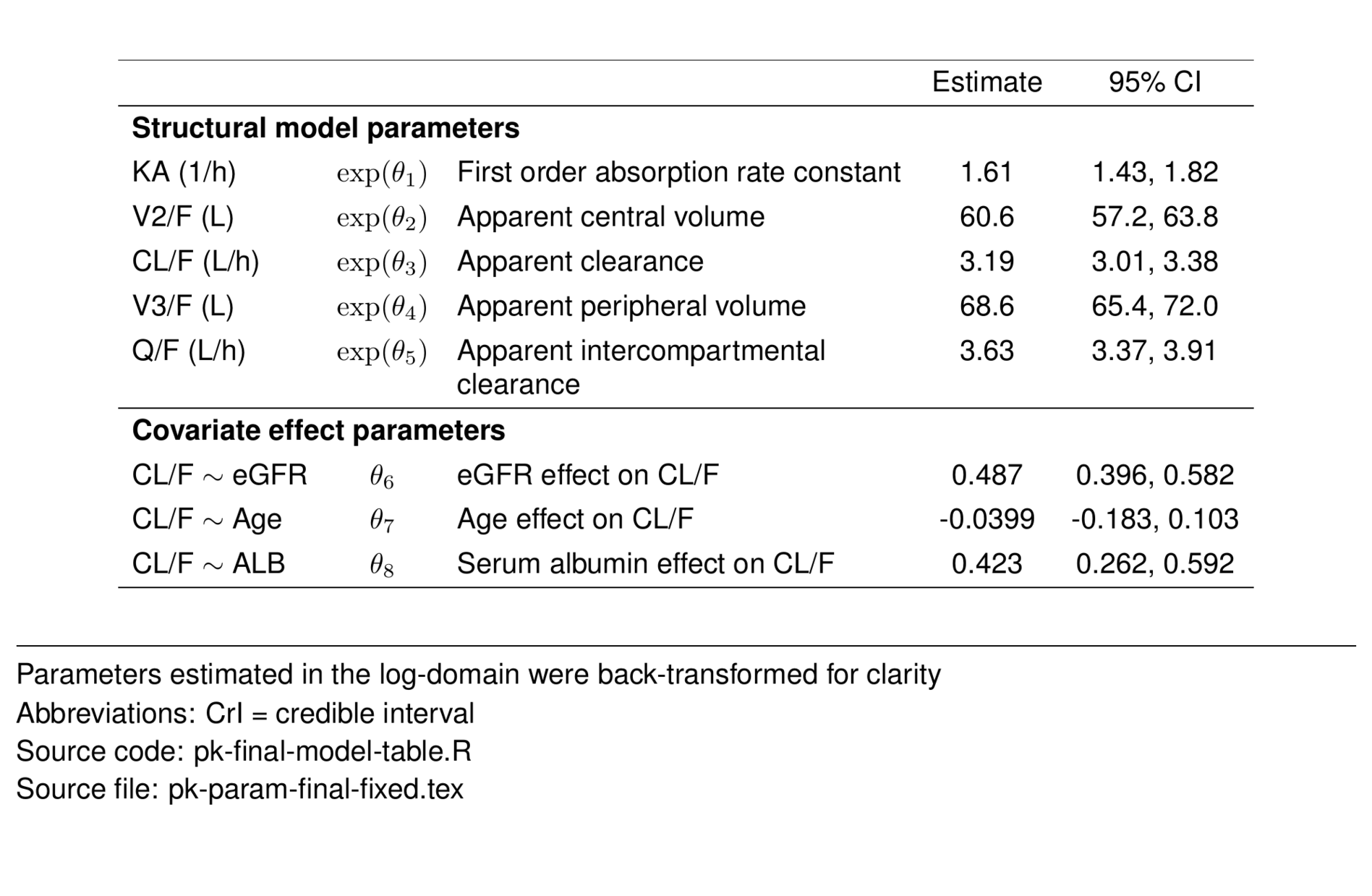
Random effect parameter table
random <- param_df %>%
  filter(str_detect(greek, "Omega") |
           str_detect(type, "Resid")) %>%
  select(-desc, -rhat, -ess_bulk, -ess_tail) %>%
  st_new %>%
  st_panel("type") %>%
  st_center(abb = "l") %>%
  st_blank("abb", "greek") %>%
  st_rename("Estimate" = "value",
            "95\\% CrI" = "ci",
            "Shrinkage (\\%)" = "shrinkage") %>%
  st_files(output = "pk-param-final-random.tex") %>%
  st_notes("Abbreviations: CrI = credible interval;
                        Corr = Correlation coefficient;
                        CV = coefficient of variation") %>%
  st_notes("CV\\% of log-normal omegas = sqrt(exp(estimate) - 1) $\\cdot$ 100") %>%
  st_notes("CV\\% of sigma = sqrt(estimate) $\\cdot$ 100") %>%
  st_noteconf(type = "minipage", width = 1) %>%
  stable() %>%
  stable_save()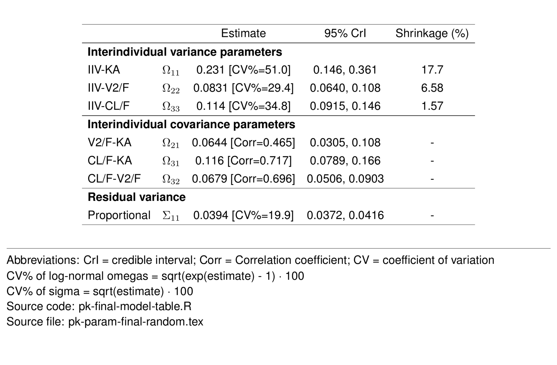
Create tex versions of the MCMC diagnostic tables
We now use the same data frame to generate tables showing the MCMC diagnostics. The meaning and interpretation of these diagnostics are described in the following publication:
Johnston CK, Waterhouse T, Wiens M, Mondick J, French J, Gillespie WR. Bayesian estimation in NONMEM. CPT Pharmacometrics Syst Pharmacol. 2023; 00: 1-16. doi.org/10.1002/psp4.13088
MCMC diagnostics: Fixed effect parameters
fixed_mcmc <- param_df %>%
  filter(str_detect(type, "Struct") |
           str_detect(type, "effect")) %>%
  select(-shrinkage, -value, -ci) %>%
  st_new() %>%
  st_panel("type") %>%
  st_center(desc = col_ragged(5.5),
            abb = "l") %>%
  st_blank("abb", "greek", "desc") %>%
  st_rename("$\\hat{R}$" = "rhat",
            "ESS bulk" = "ess_bulk",
            "ESS tail" = "ess_tail") %>%
  st_files(output = "pk-param-final-fixed-mcmc.tex") %>%
  st_notes("Abbreviations:
           ESS = effective sample size;
           $\\hat{R}$ = Gelman-Rubin diagnostic") %>%
  st_noteconf(type = "minipage", width = 1) %>%
  stable() %>%
  stable_save()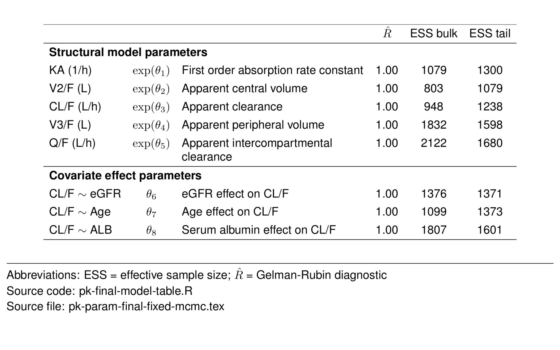
MCMC diagnostics: Random effect parameters
random_mcmc <- param_df %>%
  filter(str_detect(greek, "Omega") |
           str_detect(type, "Resid")) %>%
  select(-desc, -shrinkage, -value, -ci) %>%
  st_new %>%
  st_panel("type") %>%
  st_center(abb = "l") %>%
  st_blank("abb", "greek") %>%
  st_rename("$\\hat{R}$" = "rhat",
            "ESS bulk" = "ess_bulk",
            "ESS tail" = "ess_tail") %>%
  st_files(output = "pk-param-final-random-mcmc.tex") %>%
  st_notes("Abbreviations:
           ESS = effective sample size;
           $\\hat{R}$ = Gelman-Rubin diagnostic") %>%
  st_noteconf(type = "minipage", width = 1) %>%
  stable() %>%
  stable_save()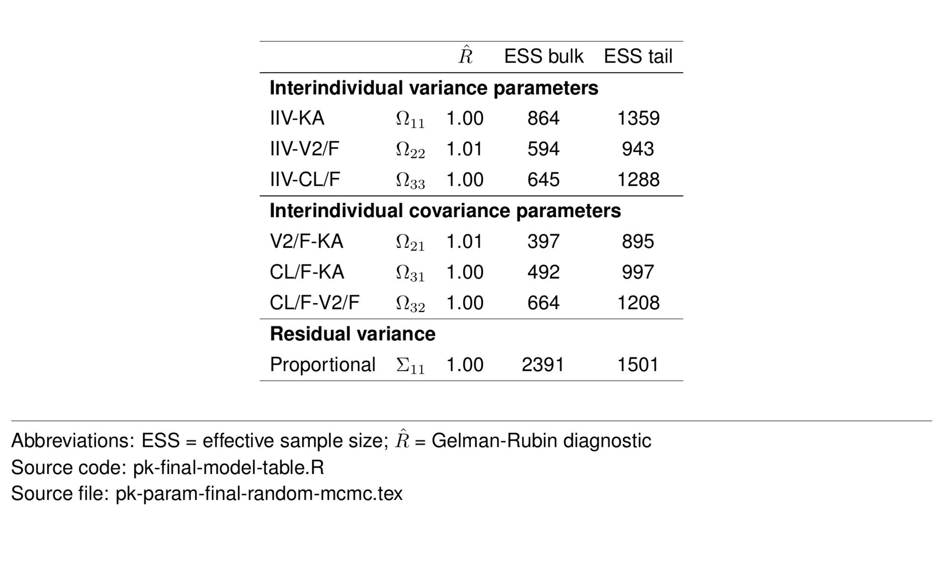
Other resources
The following scripts from the GitHub repository are discussed on this page. If you’re interested running this code, visit the About the GitHub Repo page first.
pk-base-model-table.R- creates a parameter table for the base modelpk-final-model-table.R- creates a parameter table for the final modelpk-parameter-key.yaml- parameter key for all tables