library(bbr)
library(bbr.bayes)
library(here)
library(tidyverse)
library(yspec)
library(pmforest)
library(cmdstanr)
library(posterior)
library(bayesplot)
library(tidybayes)
library(glue)
library(kableExtra)
library(jsonlite)

set_cmdstan_path(path = here("Torsten", "v0.91.0", "cmdstan"))

MODEL_DIR <- here("model", "stan")
FIGURE_DIR <- here("deliv", "figure")Introduction
Compared with specialized pharmacometrics tools, such as NONMEM®, Stan/Torsten is particularly well suited for cases where more flexibility is desired. This includes models with
- random-effects distributions other than normal
- prior distributions other than the limited set available in existing pharmacometrics tools
- multiple submodels with different random-effect structures
In this section, we illustrate the use of prior distributions that cannot be implemented in NONMEM®, specifically, spike-and-slab priors for covariate regression coefficients.
Regularized regression using shrinkage priors, such as horseshoe or spike-and-slab priors, for regression coefficients is an approach for implementing models with a large number of potential covariate effects [Piironen & Vehtari 2017, George & McCulloch 1993, Garcia & Rogers 2023]. For this Expo, we limit ourselves to the use of spike-and-slab priors for covariate effects on clearance. More realistically, we would also apply the shrinkage priors to covariate effects on other pharmacokinetic (PK) parameters.
The page demonstrates how to:
- Revise Stan/Torsten population PK (popPK) models to use spike-and-slab priors for covariate regression coefficients.
Tools used
# MetrumRG packages bbr Manage, track, and report modeling activities, through simple R objects, with a user-friendly interface between R and NONMEM®. bbr.bayes Extension of the bbr package to support Bayesian modeling with Stan or NONMEM®.
CRAN packages
dplyr A grammar of data manipulation.
Set up
Load required packages and set file paths to your model and figure directories.
Spike-and-slab priors for covariate effects
Spike-and-slab priors are shrinkage priors in the sense that they shrink “weak” regression coefficients towards zero. The type of spike-and-slab we use here constructs the prior for each regression coefficient as a mixture of two normal distributions with different variances. The “spike” is a distribution concentrated near to zero (i.e., a normal with mean zero and a small variance). The “slab” is a distribution spread over the range of plausible values (i.e., a normal with mean zero and a relatively large variance).
The overall approach is a variation on the full covariate modeling method [citation] that uses the spike-and-slab priors to stabilize the estimation process by shrinking negligible covariate effects towards the spike while applying minimal regularization to non-negligible covariate effects.
The spike-and-slab prior distribution has the following form for each covariate coefficient:
\[\begin{align} \beta_x &\sim \lambda N\left(0, \sigma_\text{slab}\right) + \left(1 - \lambda\right) N\left(0, \sigma_\text{spike}\right) \\ \lambda &\sim \text{beta}\left(a, b\right) \end{align}\]
For our example, all of the covariate coefficients share the same hyperparameters: \(\sigma\text{spike}\), \(\sigma\text{slab}\), \(a\) and \(b\). This is reasonable if we normalize the covariates in some way. Let’s normalize them by centering them about suitable reference values and dividing them by their observed sample standard deviations, i.e:
\[\begin{align} \text{EGFR}_\text{norm} &= \frac{\log\left(\text{EGFR}/90\right)}{sd\left(\log\left(\text{EGFR}\right)\right)} \\ \text{age}_\text{norm} &= \frac{\log\left(\text{age}/35\right)}{sd\left(\log\left(\text{age}\right)\right)} \\ \text{albumin}_\text{norm} &= \frac{\log\left(\text{albumin}/4.5\right)}{sd\left(\log\left(\text{albumin}\right)\right)} \\ \text{AAG}_\text{norm} &= \frac{\log\left(\text{AAG}/85\right)}{sd\left(\log\left(\text{AAG}\right)\right)} \\ \text{AST}_\text{norm} &= \frac{\log\left(\text{AST}/25\right)}{sd\left(\log\left(\text{AST}\right)\right)} \\ \text{ALT}_\text{norm} &= \frac{\log\left(\text{ALT}/22\right)}{sd\left(\log\left(\text{ALT}\right)\right)} \end{align}\]
\(\sigma_\text{spike} = 0.06\) corresponds to a 95% credible interval (CI) of \(\left(0.79, 1.27\right)\) for the ratio of individual clearance to the population typical value due to the effect of a two standard deviation difference in a covariate. That seems consistent with the notion of a negligible covariate effect. For \(\sigma_\text{slab}\), let’s choose a value that permits a plausible range of values. Using the same logic as we did for \(\sigma_\text{spike}\), \(\sigma_\text{slab} = 0.5\) results in a 95% CI of \(\left(0.095, 10.5\right)\) for the ratio of individual clearance to the typical population value due to the effects of a two standard deviation difference in a covariate. That corresponds to an extreme covariate effect. Finally, we need to choose the hyperparameters (\(a\) and \(b\)) for the prior distribution of the mixing parameter \(\lambda\). Let’s go with a value of 1 for both hyperparameters, resulting in a uniform distribution.
Model creation and submission
We construct the Stan model ppkexpo6 by building on model ppkexpo4.
ppkexpo4 <- read_model(here(MODEL_DIR, "ppkexpo4"))
ppkexpo6 <- copy_model_from(ppkexpo4, "ppkexpo6", .inherit_tags = TRUE,
                      .overwrite = TRUE) %>%
  add_description("PopPK model: ppkexpo4 plus additional covariates & spike-and-slab priors")
Now, manually edit ppkexpo6.stan to add additional covariates and incorporate spike-and-slab priors.
Here, we copy previously created files from the demo folder.
ppkexpo6 <- ppkexpo6 %>%
  add_stanmod_file(here(MODEL_DIR, "demo", "ppkexpo6.stan")) %>%
  add_standata_file(here(MODEL_DIR, "demo", "ppkexpo6-standata.R")) %>%
  add_staninit_file(here(MODEL_DIR, "demo", "ppkexpo6-init.R"))
The resulting Stan model ppkexpo6:
. /*
. Final PPK model
.   - Linear 2 compartment
.   - Non-centered parameterization
.   - lognormal residual variation
.   - Allometric scaling
.   - Additional covariates: EGFR, age, albumin, sex, AAG, AST
.   - Spike & slab priors for covariate effects
.
. Based on NONMEM PopPK FOCE example project
. */
.
. data{
.   int<lower = 1> nId; // number of individuals
.   int<lower = 1> nt; // number of events (rows in data set)
.   int<lower = 1> nObs; // number of PK observations
.   array[nObs] int<lower = 1> iObs; // event indices for PK observations
.   int<lower = 1> nBlq; // number of BLQ observations
.   array[nBlq] int<lower = 1> iBlq; // event indices for BLQ observations
.   array[nt] real<lower = 0> amt, time;
.   array[nt] int<lower = 1> cmt;
.   array[nt] int<lower = 0> evid;
.   array[nId] int<lower = 1> start, end; // indices of first & last observations
.   vector<lower = 0>[nId] weight, EGFR, age, albumin, AAG, AST, ALT;
.   vector<lower = 0, upper = 1>[nId] sex; // 0 = male, 1 = female
.   vector<lower = 0>[nObs] cObs;
.   real<lower = 0> LOQ;
. }
.
. transformed data{
.   int<lower = 1> nRandom = 5, nCmt = 3, nCov = 7;
.   array[nt] real<lower = 0> rate = rep_array(0.0, nt),
.                             ii = rep_array(0.0, nt);
.   array[nt] int<lower = 0> addl = rep_array(0, nt),
.                            ss = rep_array(0, nt);
.   array[nId, nCmt] real F = rep_array(1.0, nId, nCmt),
.                         tLag = rep_array(0.0, nId, nCmt);
.   real<lower = 0> sd_slab = 0.5, sd_spike = 0.06,
.                   alpha_mix = 1, beta_mix = 1;
.   vector[nId] logEGFR_norm = log(EGFR / 90) / sd(log(EGFR));
.   vector[nId] logage_norm = log(age / 35) / sd(log(age));
.   vector[nId] logalbumin_norm = log(albumin / 4.5) / sd(log(albumin));
.   vector[nId] logAAG_norm = log(AAG / 85) / sd(log(AAG));
.   vector[nId] logAST_norm = log(AST / 25) / sd(log(AST));
.   vector[nId] logALT_norm = log(ALT / 22) / sd(log(ALT));
. }
.
. parameters{
.   real<lower = 0> CLHat, QHat, V2Hat, V3Hat;
. // To constrain kaHat > lambda1 uncomment the following
.   real<lower = (CLHat / V2Hat + QHat / V2Hat + QHat / V3Hat +
.       sqrt((CLHat / V2Hat + QHat / V2Hat + QHat / V3Hat)^2 -
.            4 * CLHat / V2Hat * QHat / V3Hat)) / 2> kaHat; // ka > lambda_1
.   real EGFR_CL, age_CL, albumin_CL, sex_CL, AAG_CL, AST_CL, ALT_CL;
.   real<lower = 0, upper = 1> lambda_mix;
. //    vector<lower = 0, upper = 1>[nCov] lambda_mix;
.
.   real<lower = 0> sigma;
.   vector<lower = 0>[nRandom] omega;
.   cholesky_factor_corr[nRandom] L_corr;
.   matrix[nRandom, nId] z;
. }
.
. transformed parameters{
.   vector[nRandom] thetaHat = log([CLHat, QHat, V2Hat, V3Hat, kaHat]');
.   // Individual parameters
.   matrix[nId, nRandom] theta = (rep_matrix(thetaHat, nId) + diag_pre_multiply(omega, L_corr * z))';
.   vector<lower = 0>[nId] CL = exp(theta[,1] + 0.75 * log(weight / 70) +
.                               EGFR_CL * logEGFR_norm +
.                               age_CL * logage_norm +
.                               albumin_CL * logalbumin_norm +
.                               sex_CL * sex +
.                               AAG_CL * logAAG_norm +
.                               AST_CL * logAST_norm +
.                               ALT_CL * logALT_norm),
.                          Q = exp(theta[,2] + 0.75 * log(weight / 70)),
.                          V2 = exp(theta[,3] + log(weight / 70)),
.                          V3 = exp(theta[,4] + log(weight / 70)),
.                          ka = exp(theta[,5]);
.   corr_matrix[nRandom] rho =  L_corr * L_corr';
.
.   row_vector[nt] cHat; // predicted concentration
.   matrix[nCmt, nt] x; // mass in all compartments
.
.   for(j in 1:nId){
.     x[, start[j]:end[j]] = pmx_solve_twocpt(time[start[j]:end[j]],
.                                             amt[start[j]:end[j]],
.                                             rate[start[j]:end[j]],
.                                             ii[start[j]:end[j]],
.                                             evid[start[j]:end[j]],
.                                             cmt[start[j]:end[j]],
.                                             addl[start[j]:end[j]],
.                                             ss[start[j]:end[j]],
.                                             {CL[j], Q[j], V2[j], V3[j], ka[j]});
.
.     cHat[start[j]:end[j]] = x[2, start[j]:end[j]] / V2[j];
.   }
. }
.
. model{
.   // priors
.   CLHat ~ normal(0, 10);
.   QHat ~ normal(0, 10);
.   V2Hat ~ normal(0, 50);
.   V3Hat ~ normal(0, 100);
.   kaHat ~ normal(0, 3);
.
.   // spike & slab priors
.   lambda_mix ~ beta(alpha_mix, beta_mix);
.   target += log_mix(lambda_mix,
.                     normal_lpdf(EGFR_CL | 0, sd_slab),
.                     normal_lpdf(EGFR_CL | 0, sd_spike));
.   target += log_mix(lambda_mix,
.                     normal_lpdf(age_CL | 0, sd_slab),
.                     normal_lpdf(age_CL | 0, sd_spike));
.   target += log_mix(lambda_mix,
.                     normal_lpdf(albumin_CL | 0, sd_slab),
.                     normal_lpdf(albumin_CL | 0, sd_spike));
.   target += log_mix(lambda_mix,
.                     normal_lpdf(sex_CL | 0, sd_slab),
.                     normal_lpdf(sex_CL | 0, sd_spike));
.   target += log_mix(lambda_mix,
.                     normal_lpdf(AAG_CL | 0, sd_slab),
.                     normal_lpdf(AAG_CL | 0, sd_spike));
.   target += log_mix(lambda_mix,
.                     normal_lpdf(AST_CL | 0, sd_slab),
.                     normal_lpdf(AST_CL | 0, sd_spike));
.   target += log_mix(lambda_mix,
.                     normal_lpdf(ALT_CL | 0, sd_slab),
.                     normal_lpdf(ALT_CL | 0, sd_spike));
.
.   sigma ~ normal(0, 0.5);
.   omega ~ normal(0, 0.5);
.   L_corr ~ lkj_corr_cholesky(2);
.
.   // interindividual variability
.   to_vector(z) ~ normal(0, 1);
.
.   // likelihood
.   cObs ~ lognormal(log(cHat[iObs]), sigma); // observed data likelihood
.   target += lognormal_lcdf(LOQ | log(cHat[iBlq]), sigma); // BLQ data likelihood
.
. }
.
. generated quantities{
.   // Individual parameters for hypothetical new individuals
.   matrix[nRandom, nId] zNew;
.   matrix[nId, nRandom] thetaNew;
.   vector<lower = 0>[nId] CLNew, QNew, V2New, V3New, kaNew;
.
.   row_vector[nt] cHatNew; // predicted concentration in new individuals
.   matrix[nCmt, nt] xNew; // mass in all compartments in new individuals
.   array[nt] real cPred, cPredNew;
.
.   vector[nObs + nBlq] log_lik;
.
.   // Simulations for posterior predictive checks
.   for(j in 1:nId){
.     zNew[,j] = to_vector(normal_rng(rep_vector(0, nRandom), 1));
.   }
.   thetaNew = (rep_matrix(thetaHat, nId) + diag_pre_multiply(omega, L_corr * zNew))';
.   CLNew = exp(thetaNew[,1] + 0.75 * log(weight / 70) +
.                              EGFR_CL * logEGFR_norm +
.                              age_CL * logage_norm +
.                              albumin_CL * logalbumin_norm +
.                              sex_CL * sex +
.                              AAG_CL * logAAG_norm +
.                              AST_CL * logAST_norm +
.                              ALT_CL * logALT_norm);
.   QNew = exp(thetaNew[,2] + 0.75 * log(weight / 70));
.   V2New = exp(thetaNew[,3] + log(weight / 70));
.   V3New = exp(thetaNew[,4] + log(weight / 70));
.   kaNew = exp(thetaNew[,5]);
.
.   for(j in 1:nId){
.     xNew[, start[j]:end[j]] = pmx_solve_twocpt(time[start[j]:end[j]],
.                                                amt[start[j]:end[j]],
.                                                rate[start[j]:end[j]],
.                                                ii[start[j]:end[j]],
.                                                evid[start[j]:end[j]],
.                                                cmt[start[j]:end[j]],
.                                                addl[start[j]:end[j]],
.                                                ss[start[j]:end[j]],
.                                                {CLNew[j], QNew[j], V2New[j],
.                                                V3New[j], kaNew[j]});
.
.     cHatNew[start[j]:end[j]] = xNew[2, start[j]:end[j]] / V2New[j];
.
.
.     cPred[start[j]] = 0.0;
.     cPredNew[start[j]] = 0.0;
.     // new observations in existing individuals
.     cPred[(start[j] + 1):end[j]] = lognormal_rng(log(cHat[(start[j] + 1):end[j]]),
.       sigma);
.     // new observations in new individuals
.     cPredNew[(start[j] + 1):end[j]] = lognormal_rng(log(cHatNew[(start[j] + 1):end[j]]),
.       sigma);
.   }
.
.   // Calculate log-likelihood values to use for LOO CV
.
.   // Observation-level log-likelihood
.   for(i in 1:nObs)
.     log_lik[i] = lognormal_lpdf(cObs[i] | log(cHat[iObs[i]]), sigma);
.   for(i in 1:nBlq)
.     log_lik[i + nObs] = lognormal_lcdf(LOQ | log(cHat[iBlq[i]]), sigma);
.
. }
ppkexpo6: Submit the model
## Set cmdstanr arguments
ppkexpo6 <- ppkexpo6 %>%
  set_stanargs(list(iter_warmup = 500,
                    iter_sampling = 500,
                    thin = 1,
                    chains = 4,
                    parallel_chains = 4,
                    seed = 1234,
                    save_warmup = FALSE),
               .clear = TRUE)

## Fit the model using Stan
ppkexpo6_fit <- ppkexpo6 %>% submit_model(.overwrite = TRUE)
ppkexpo6: Parameter summary and sampling diagnostics
model_name <- "ppkexpo6"
mod <- read_model(here(MODEL_DIR, model_name))
fit <- read_fit_model(mod)

fit$cmdstan_diagnose()
. Processing csv files: /data/expos/expo4-torsten-poppk/model/stan/ppkexpo6/ppkexpo6-output/ppkexpo6-202408212022-1-6611b8.csv, /data/expos/expo4-torsten-poppk/model/stan/ppkexpo6/ppkexpo6-output/ppkexpo6-202408212022-2-6611b8.csv, /data/expos/expo4-torsten-poppk/model/stan/ppkexpo6/ppkexpo6-output/ppkexpo6-202408212022-3-6611b8.csv, /data/expos/expo4-torsten-poppk/model/stan/ppkexpo6/ppkexpo6-output/ppkexpo6-202408212022-4-6611b8.csv
.
. Checking sampler transitions treedepth.
. Treedepth satisfactory for all transitions.
.
. Checking sampler transitions for divergences.
. No divergent transitions found.
.
. Checking E-BFMI - sampler transitions HMC potential energy.
. E-BFMI satisfactory.
.
. Effective sample size satisfactory.
.
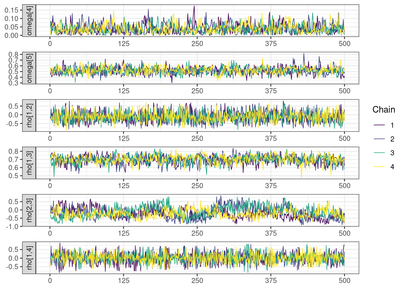
. The following parameters had split R-hat greater than 1.05:
. L_corr[3,2], L_corr[5,2], z[2,104], z[2,152], rho[3,2], rho[2,3]
. Such high values indicate incomplete mixing and biased estimation.
. You should consider regularizating your model with additional prior information or a more effective parameterization.
.
. Processing complete.pars <- c("lp__", "CLHat", "QHat", "V2Hat", "V3Hat", "kaHat",
"EGFR_CL", "age_CL", "albumin_CL", "sex_CL", "AAG_CL",
"AST_CL", "ALT_CL", "lambda_mix",
"sigma", glue("omega[{1:5}]"),
paste0("rho[", matrix(apply(expand.grid(1:5, 1:5),
1, paste, collapse = ","),
ncol = 5)[upper.tri(diag(5),
diag = FALSE)], "]"))
# Get posterior samples for parameters of interest
posterior <- fit$draws(variables = pars)
# Get quantities related to NUTS performance, e.g., occurrence of
# divergent transitions
np <- nuts_params(fit)
n_iter <- dim(posterior)[1]
n_chains <- dim(posterior)[2]
ptable <- fit$summary(variables = pars) %>%
mutate(across(-variable, ~ pmtables::sig(.x, maxex = 4))) %>%
rename(parameter = variable) %>%
mutate("90% CI" = paste("(", q5, ", ", q95, ")",
sep = "")) %>%
select(parameter, mean, median, sd, mad, "90% CI", ess_bulk, ess_tail, rhat)
ptable %>%
kable %>%
kable_styling()| parameter | mean | median | sd | mad | 90% CI | ess_bulk | ess_tail | rhat |
|---|---|---|---|---|---|---|---|---|
| lp__ | -28.0 | -28.5 | 26.4 | 26.5 | (-71.8, 14.9) | 449 | 894 | 1.00 |
| CLHat | 3.37 | 3.37 | 0.116 | 0.112 | (3.19, 3.56) | 249 | 387 | 1.02 |
| QHat | 3.75 | 3.75 | 0.153 | 0.148 | (3.51, 4.01) | 1590 | 1770 | 1.01 |
| V2Hat | 61.7 | 61.7 | 1.82 | 1.79 | (58.9, 64.8) | 465 | 819 | 1.01 |
| V3Hat | 67.7 | 67.6 | 1.52 | 1.54 | (65.2, 70.2) | 3760 | 1680 | 1.00 |
| kaHat | 1.64 | 1.63 | 0.116 | 0.113 | (1.46, 1.84) | 807 | 1270 | 1.01 |
| EGFR_CL | 0.214 | 0.214 | 0.0226 | 0.0226 | (0.178, 0.252) | 452 | 688 | 1.01 |
| age_CL | -0.0126 | -0.0129 | 0.0202 | 0.0205 | (-0.0462, 0.0195) | 421 | 714 | 1.01 |
| albumin_CL | 0.0945 | 0.0951 | 0.0217 | 0.0210 | (0.0589, 0.129) | 472 | 771 | 1.00 |
| sex_CL | -0.0143 | -0.0142 | 0.0325 | 0.0322 | (-0.0678, 0.0394) | 567 | 914 | 1.00 |
| AAG_CL | 0.0143 | 0.0145 | 0.0193 | 0.0197 | (-0.0181, 0.0461) | 499 | 814 | 1.01 |
| AST_CL | 0.0557 | 0.0560 | 0.0200 | 0.0205 | (0.0220, 0.0879) | 465 | 871 | 1.01 |
| ALT_CL | 0.000513 | 0.000518 | 0.0194 | 0.0191 | (-0.0323, 0.0319) | 423 | 618 | 1.01 |
| lambda_mix | 0.258 | 0.235 | 0.163 | 0.161 | (0.0373, 0.575) | 3510 | 1050 | 1.00 |
| sigma | 0.213 | 0.213 | 0.00281 | 0.00271 | (0.209, 0.218) | 2570 | 1710 | 1.00 |
| omega[1] | 0.335 | 0.334 | 0.0191 | 0.0189 | (0.304, 0.367) | 302 | 838 | 1.02 |
| omega[2] | 0.0613 | 0.0526 | 0.0453 | 0.0448 | (0.00588, 0.147) | 573 | 1010 | 1.01 |
| omega[3] | 0.289 | 0.287 | 0.0206 | 0.0200 | (0.257, 0.325) | 871 | 1310 | 1.00 |
| omega[4] | 0.0398 | 0.0344 | 0.0286 | 0.0294 | (0.00404, 0.0943) | 782 | 1050 | 1.00 |
| omega[5] | 0.518 | 0.516 | 0.0623 | 0.0618 | (0.421, 0.621) | 1030 | 1460 | 1.00 |
| rho[1,2] | -0.114 | -0.136 | 0.314 | 0.328 | (-0.607, 0.447) | 2970 | 1370 | 1.00 |
| rho[1,3] | 0.697 | 0.700 | 0.0528 | 0.0534 | (0.604, 0.776) | 679 | 1210 | 1.00 |
| rho[2,3] | -0.178 | -0.212 | 0.333 | 0.349 | (-0.672, 0.425) | 63.0 | 253 | 1.05 |
| rho[1,4] | 0.00760 | 0.00692 | 0.307 | 0.318 | (-0.498, 0.533) | 4090 | 1340 | 1.00 |
| rho[2,4] | 0.00581 | -0.00783 | 0.350 | 0.394 | (-0.571, 0.587) | 2240 | 1420 | 1.00 |
| rho[3,4] | 0.0404 | 0.0446 | 0.312 | 0.330 | (-0.470, 0.540) | 3730 | 1670 | 1.00 |
| rho[1,5] | 0.673 | 0.677 | 0.0829 | 0.0854 | (0.535, 0.801) | 939 | 1180 | 1.00 |
| rho[2,5] | -0.185 | -0.216 | 0.352 | 0.379 | (-0.704, 0.459) | 88.3 | 406 | 1.05 |
| rho[3,5] | 0.511 | 0.515 | 0.0934 | 0.0963 | (0.347, 0.654) | 1110 | 1350 | 1.00 |
| rho[4,5] | -0.0525 | -0.0481 | 0.331 | 0.349 | (-0.582, 0.498) | 309 | 736 | 1.01 |
Trace and density plots
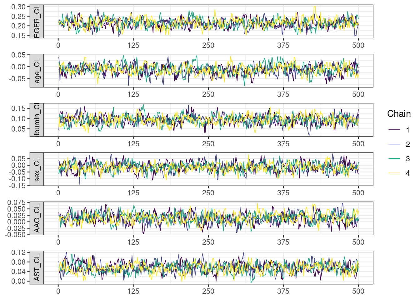
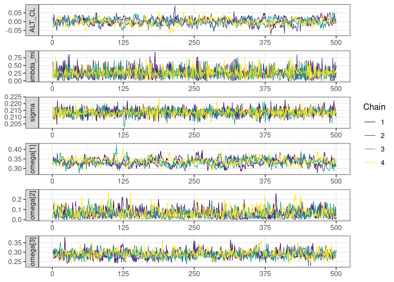
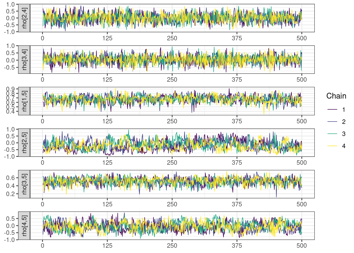
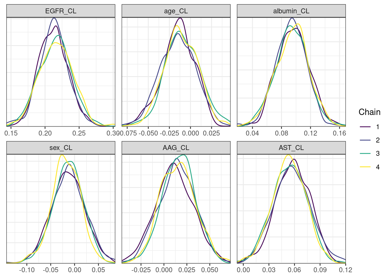
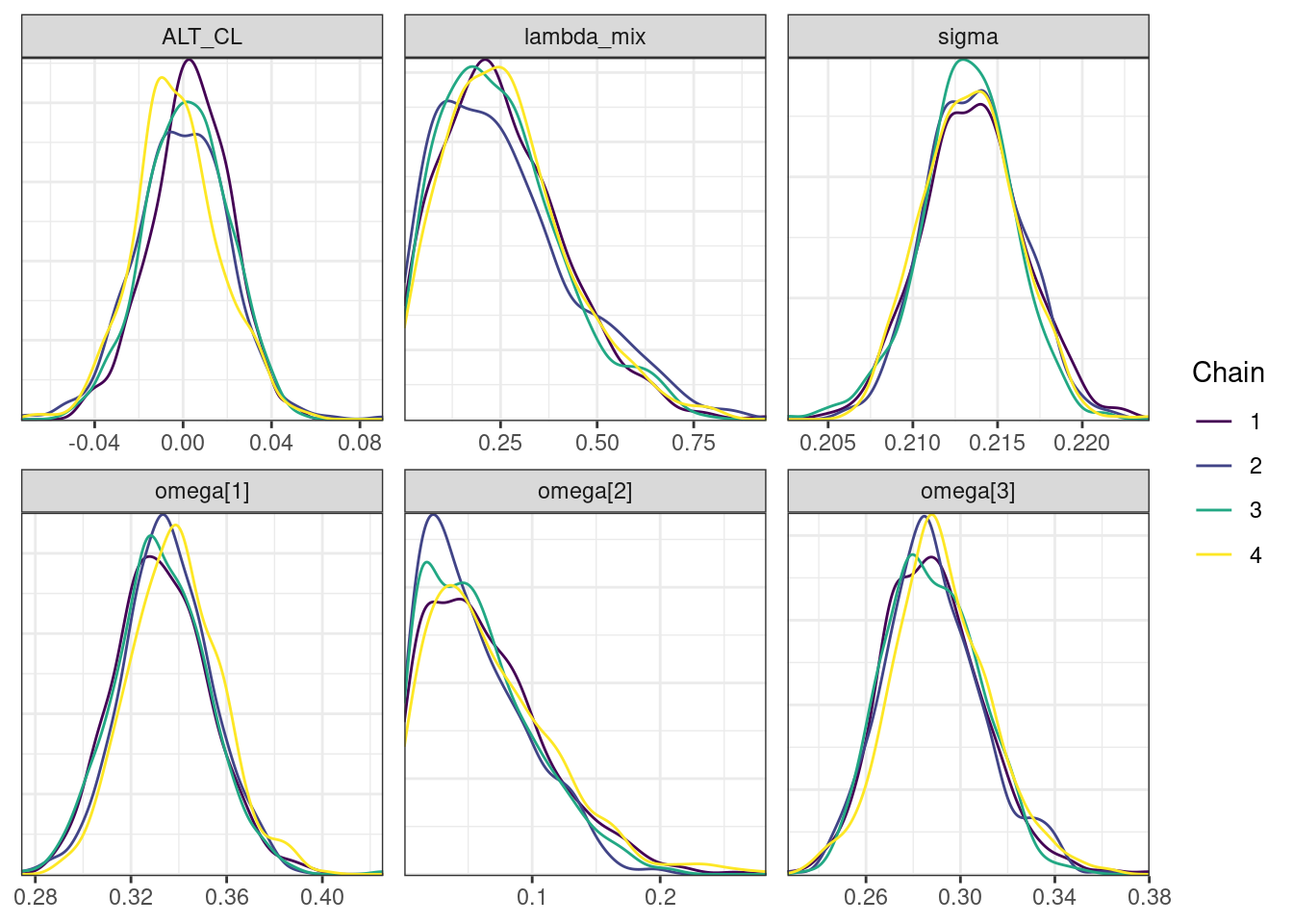
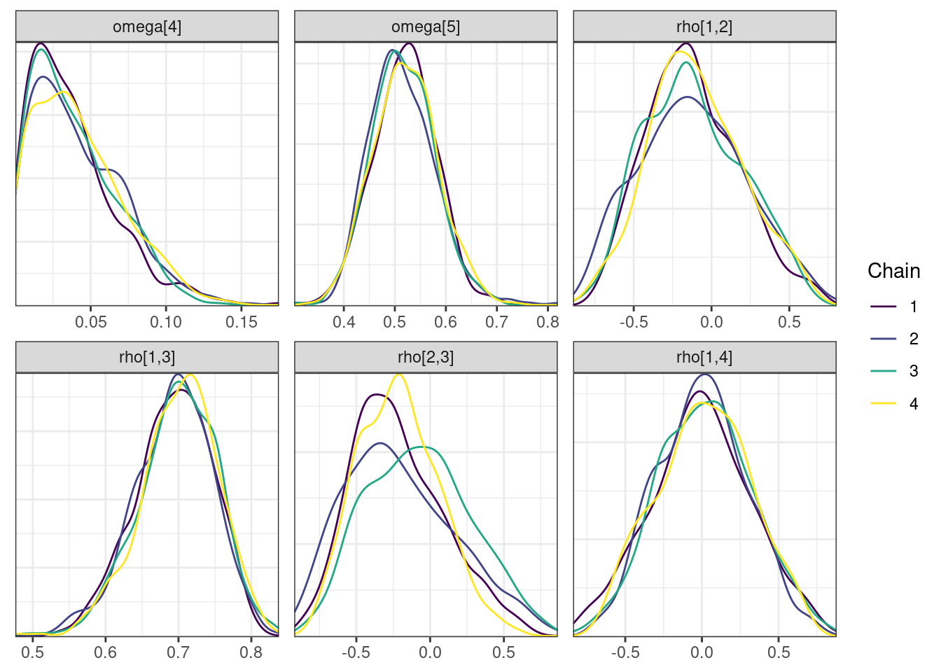
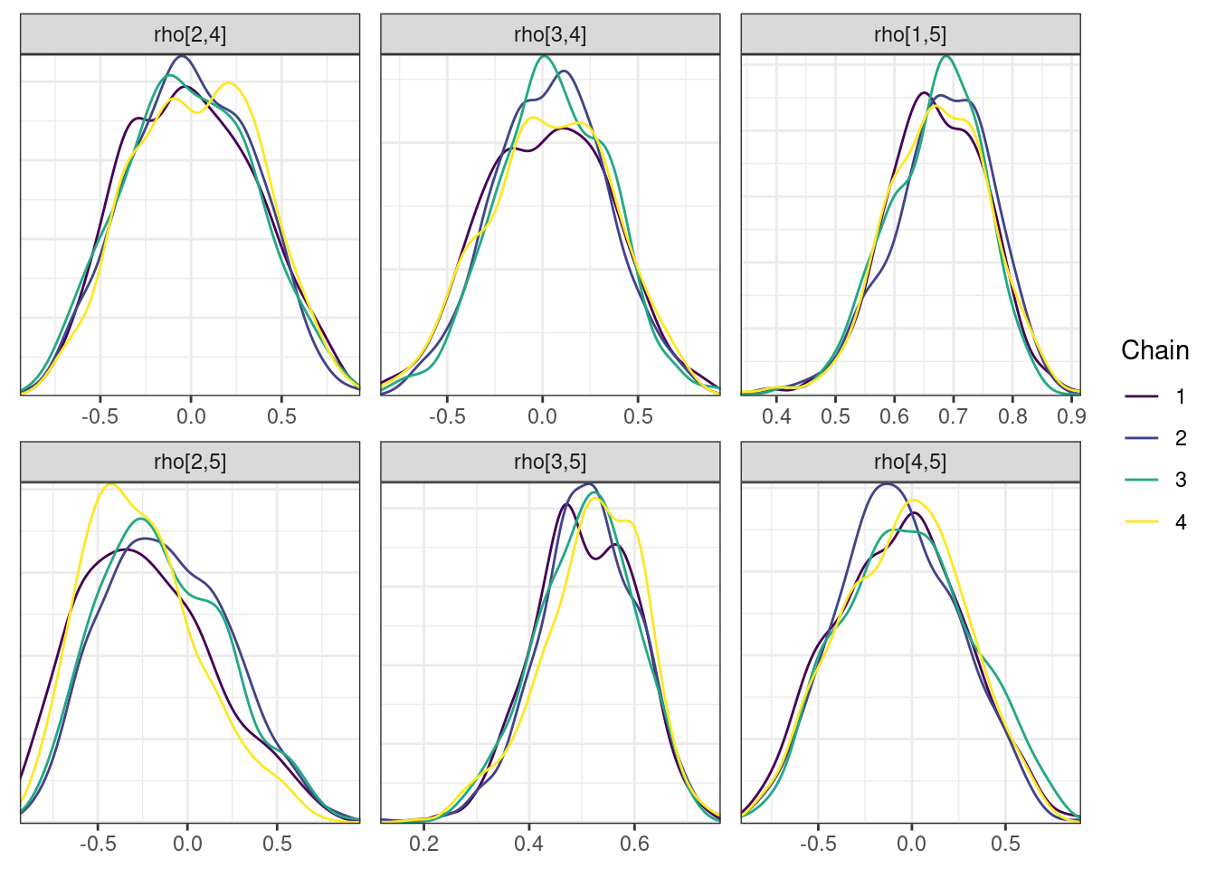
Next, we look at the trace and density plots.
mcmc_history_plots <- mcmc_history(posterior,
                                  nParPerPage = 6,
np = np)mcmc_history_plots. [[1]].
. [[2]].
. [[3]].
. [[4]].
. [[5]]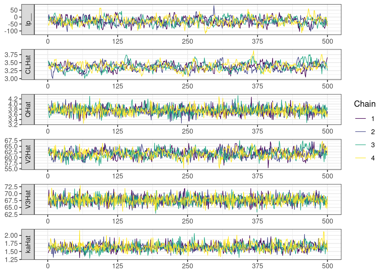
  mcmc_density_chain_plots <- mcmc_density(posterior,
nParPerPage = 6, byChain = TRUE)mcmc_density_chain_plots. [[1]].
. [[2]].
. [[3]].
. [[4]].
. [[5]]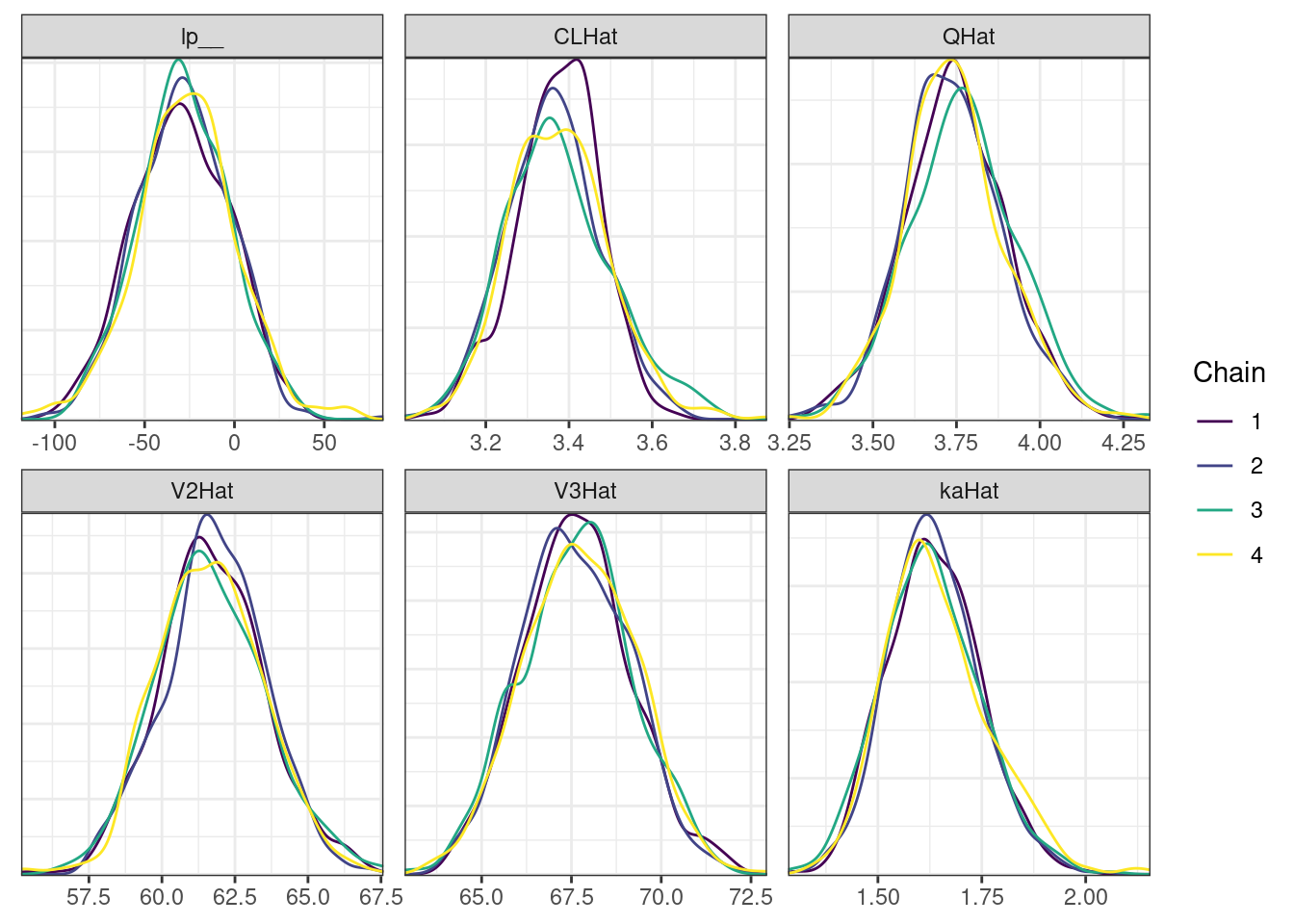
Covariate forest plots
Construct data for creating forest plots
Calculate posterior samples for “typical” clearance in reference patients and for various subgroups constructed by varying one covariate at a time.
CL_pars <- fit$draws(variables = c("EGFR_CL", "age_CL",
                                  "albumin_CL", "sex_CL", "AAG_CL",
                                  "AST_CL", "ALT_CL"),
                     format = "draws_df") %>%
  pivot_longer(cols = ends_with("_CL")) %>%
  mutate(group = str_split_i(name, "_", 1))

covariate_ranges <- data.frame(group = c("EGFR", "EGFR", "EGFR",
                                         "albumin", "albumin",
                                         "age", "age",
                                         "sex", "sex",
                                         "AAG", "AAG",
                                         "AST", "AST",
                                         "ALT", "ALT"),
                               group_level = c(22.6, 42.9, 74.9,
                                               3.25, 5,
                                               20, 45,
                                               0, 1,
                                               53, 115,
                                               11, 34,
                                               12,32))

covariates <- read_json(get_data_path(mod), simplifyVector = TRUE)
covariates <- as_tibble(covariates[c("EGFR", "age", "albumin",
                                     "AAG", "AST", "ALT")])
sd_cov <- sapply(covariates, function(x) sd(log(x)))
sd_cov <- tibble(group = names(sd_cov), sd = sd_cov)

ref <- tibble(group = c("EGFR", "age", "albumin", "AAG", "AST", "ALT"),
              ref = c(90, 35, 4.5, 85, 25, 22))

CL_sims <- covariate_ranges %>%
  left_join(ref) %>%
  left_join(sd_cov) %>%
  left_join(CL_pars)

CL_sims <- CL_sims %>%
  mutate(CLratio = if_else(group == "sex",
                           exp(value * group_level),
                           exp(value * log(group_level / ref) / sd)))

CL_summary <- summarize_data(CL_sims, value = "CLratio", group = "group",
                             group_level = "group_level")

cl_forest <- plot_forest(CL_summary,
##  summary_label = plot_labels,
  text_size = 3.5,
  vline_intercept = 1,
  x_lab = "Fraction and 95% CI \nRelative to Reference",
  CI_label = "Median [95% CI]",
  plot_width = 8,
  x_breaks = c(0.4,0.6, 0.8, 1, 1.2, 1.4,1.6),
  x_limit = c(0.4,1.45),
  annotate_CI = TRUE,
  nrow = 1
)
cl_forest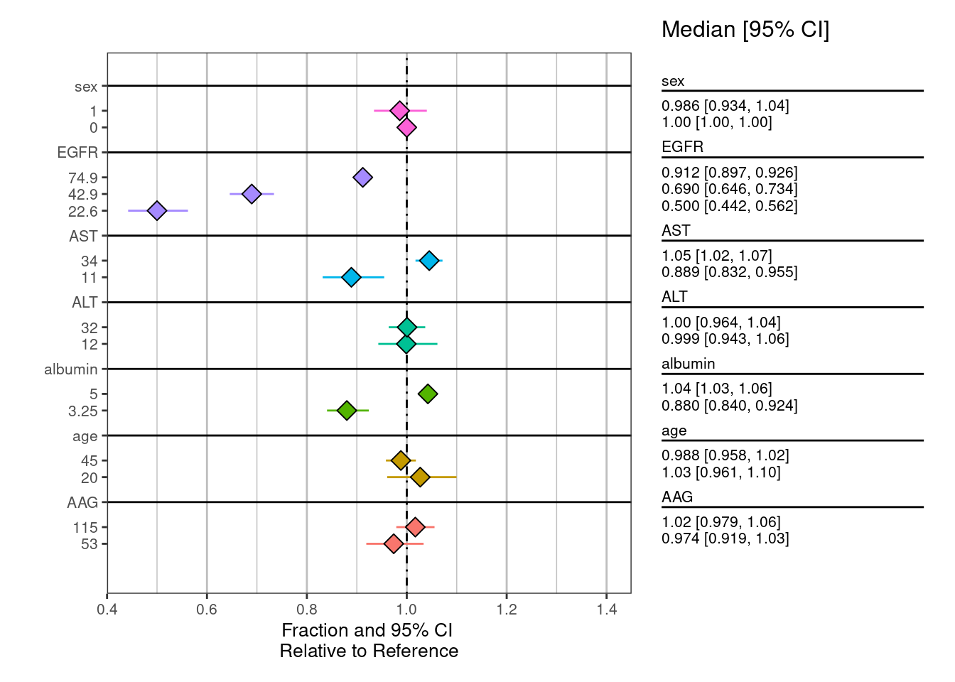
Other resources
The following script from the GitHub repository is discussed on this page. If you’re interested running this code, visit the About the GitHub Repo page first.
Shrinkage Priors script: shrinkage-priors.Rmd