Introduction

The Markov Chain Monte Carlo (MCMC) diagnostics presented in the previous section assess whether the posterior distributions of the model parameters are characterized with sufficient fidelity. If so, we can then assess the goodness-of-fit (GOF) of the model to the data which is the focus of this section. We focus on the use of posterior predictive checking (PPC)—the Bayesian (Bayes) approach to visual predictive checks (VPCs).

Tools used

MetrumRG packages

bbr Manage, track, and report modeling activities, through simple R objects, with a user-friendly interface between R and NONMEM®.

bbr.bayes Extension of the bbr package to support Bayesian modeling with Stan or NONMEM®.

CRAN packages

bayesplot Plotting Bayesian models and diagnostics with ggplot.

posterior Provides tools for working with output from Bayesian models, including output from CmdStan.

tidyvpc Create visual predictive checks using tidyverse-style syntax.

tidybayes Integrate Bayesian modeling with the tidyverse.

Set up

Load required packages and set file paths to your model and figure directories.

library(bbr)
library(bbr.bayes)
library(tidyverse)
library(here)
library(tidybayes)
library(bayesplot)
library(tidyvpc)

MODEL_DIR <- here("model", "stan")
FIGURE_DIR <- here("deliv", "figure")

bayesplot::color_scheme_set('viridis')
theme_set(theme_bw())

Get the model output

Read in the output from our first base model, ppkexpo1. This is done using the read_fit_model function from bbr.bayes which returns a CmdStanMCMC object, providing several methods for querying the fitting results. For example, fit$draws() returns a draws array containing the MCMC samples.

model_name <- "ppkexpo1"
mod <- read_model(here(MODEL_DIR, model_name))
fit <- read_fit_model(mod)

PPCs for individuals

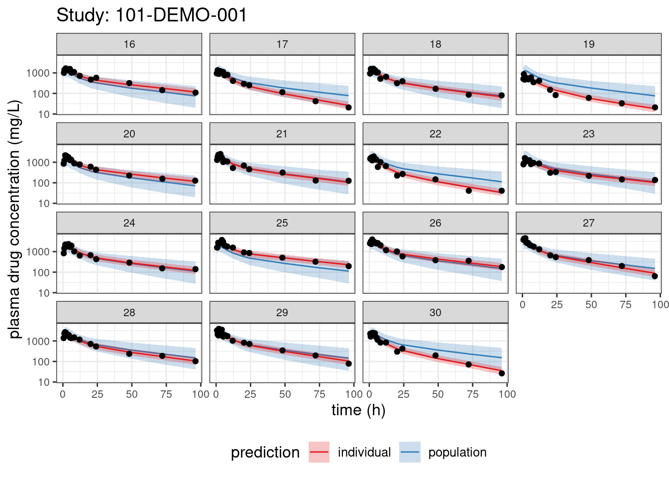
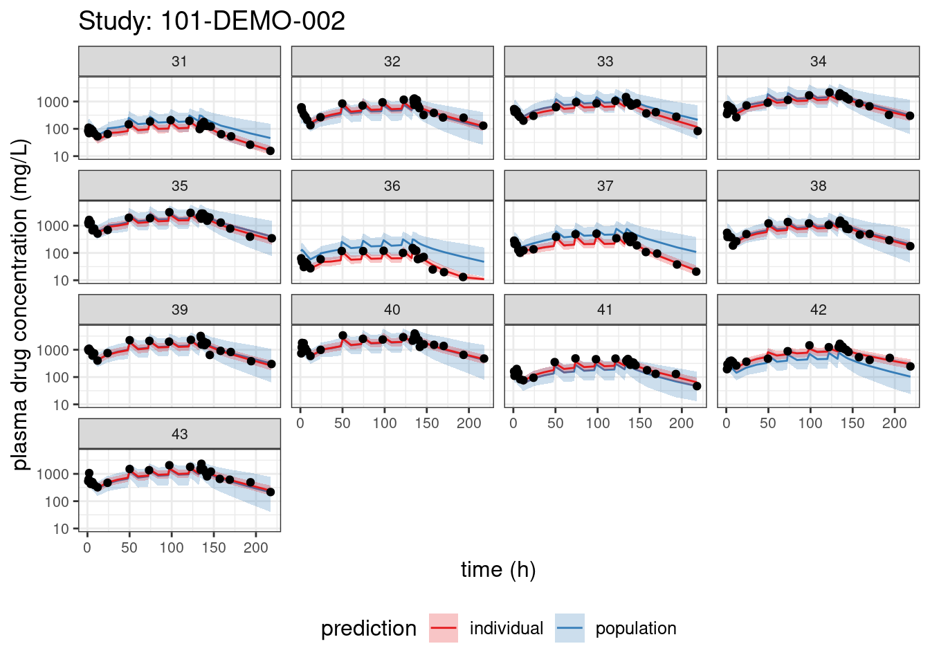
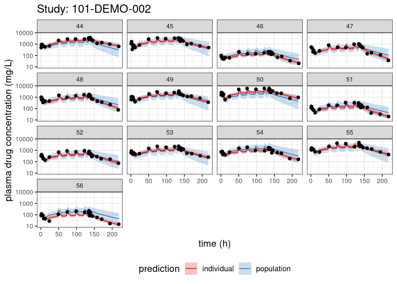
We begin with PPCs, allowing us to compare model-predicted plasma concentrations to the observed values for each individual. The resulting plots depict 90% credible intervals (CI) for the model-predicted concentrations vs time overlayed with the observed values. Two types of model predictions are shown: “individual” represents predictions of new observations in the same individual and “population” predicts new observations in new patients with the same covariate values and dosing. These are Bayesian analogs of IPRED and PRED.

load(file = here::here(dirname(get_data_path(mod)), "data1.RData"))
loq <- 10

data2 <- data1 %>%
  mutate(DV = if_else(EVID == 1, NA_real_, DV),
         DV = if_else(BLQ == 1, NA_real_, DV))

pred <- spread_draws(fit, 
                     cPred[num], 
                     cPredNew[num]) %>%
  mutate(cPred = ifelse(cPred < loq, NA_real_, cPred),
         cPredNew = ifelse(cPredNew < loq, NA_real_, cPredNew)) %>%
  group_by(num) %>%
  summarize(lb = quantile(cPred, probs = 0.05, na.rm = TRUE),
            median = quantile(cPred, probs = 0.5, na.rm = TRUE),
            ub = quantile(cPred, probs = 0.95, na.rm = TRUE),
            lbNew = quantile(cPredNew, probs = 0.05, na.rm = TRUE),
            medianNew = quantile(cPredNew, probs = 0.5, na.rm = TRUE),
            ubNew = quantile(cPredNew, probs = 0.95, na.rm = TRUE)) %>%
  left_join(data2 %>% mutate(num = 1:n()))

nPerPage <- 16
studies <- unique(data2$STUDY)
ppc_ind <- lapply(studies,
              function(thisStudy){
                predStudy <- pred %>%
                  filter(STUDY == thisStudy)
                ids <- unique(predStudy %>% dplyr::pull(ID))
                nId <- length(ids)
                nPages <- ceiling(nId / nPerPage)
                ids <- data.frame(ID = ids,
                                  page = sort(rep(1:nPages, length = nId)),
                                  stringsAsFactors = FALSE)
                predStudy <- predStudy %>%
                  left_join(ids)
                lapply(1:nPages,
                       function(thisPage){
                         predPage <- predStudy %>% filter(page == thisPage)
                         ggplot(predPage, 
                                aes(x = TIME, y = DV)) +
                           geom_line(aes(x = TIME, y = medianNew, 
                                         color = "population")) +
                           geom_ribbon(aes(ymin = lbNew, ymax = ubNew, 
                                           fill = "population"), 
                                       alpha = 0.25) +
                           geom_line(aes(x = TIME, y = median, 
                                         color = "individual")) +
                           geom_ribbon(aes(ymin = lb, ymax = ub, 
                                           fill = "individual"), 
                                       alpha = 0.25) +
                           scale_color_brewer(name  ="prediction",
                                              breaks=c("individual", "population"),
                                              palette = "Set1") +
                           scale_fill_brewer(name  ="prediction",
                                             breaks=c("individual", "population"),
                                             palette = "Set1") +
                           geom_point(na.rm = TRUE) +
                           scale_y_log10() +
                           labs(title = paste("Study:", thisStudy),
                                x = "time (h)",
                                y = "plasma drug concentration (mg/L)") +
                           theme(text = element_text(size = 12),
                                 axis.text = element_text(size = 8),
                                 legend.position = "bottom",
                                 strip.text = element_text(size = 8)) +
                           facet_wrap(~ ID)
                       })
              })

# show plot in HTML output
ppc_ind

. [[1]]
. [[1]][[1]]

. 
. [[1]][[2]]

. 
. 
. [[2]]
. [[2]][[1]]

. 
. [[2]][[2]]

. 
. [[2]][[3]]

. 
. [[2]][[4]]

. 
. 
. [[3]]
. [[3]][[1]]

. 
. [[3]][[2]]

. 
. [[3]][[3]]

. 
. 
. [[4]]
. [[4]][[1]]

. 
. [[4]][[2]]

. 
. [[4]][[3]]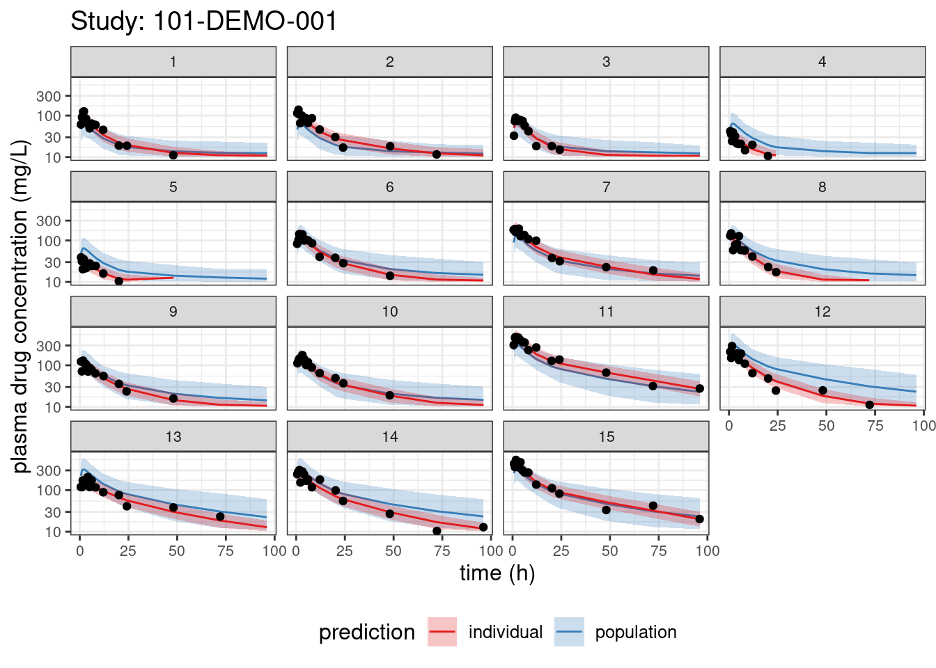

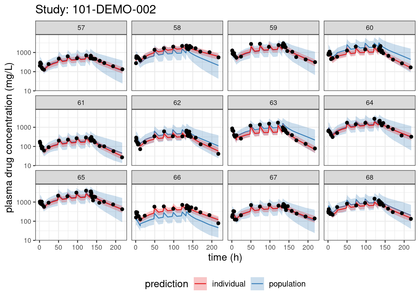
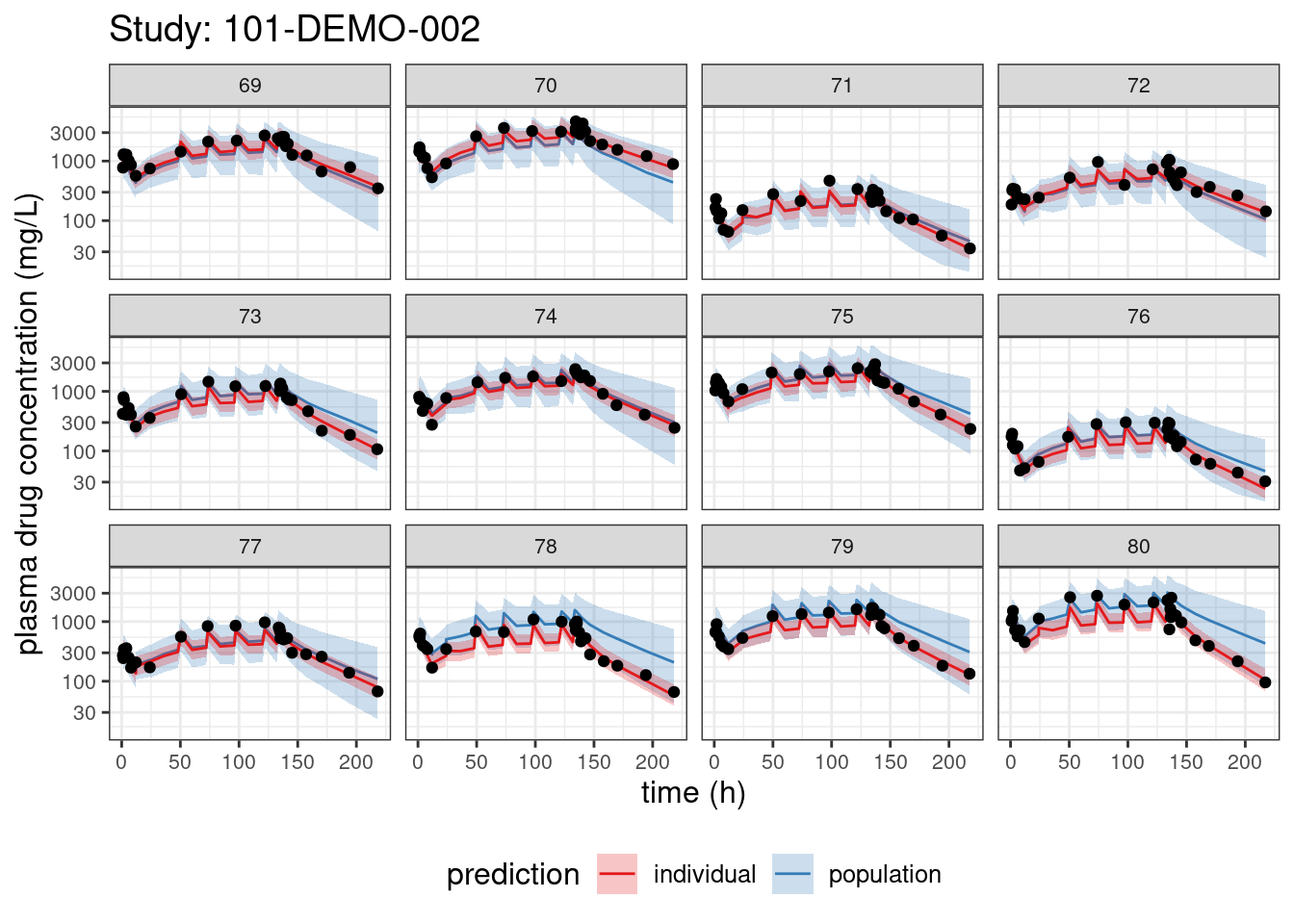
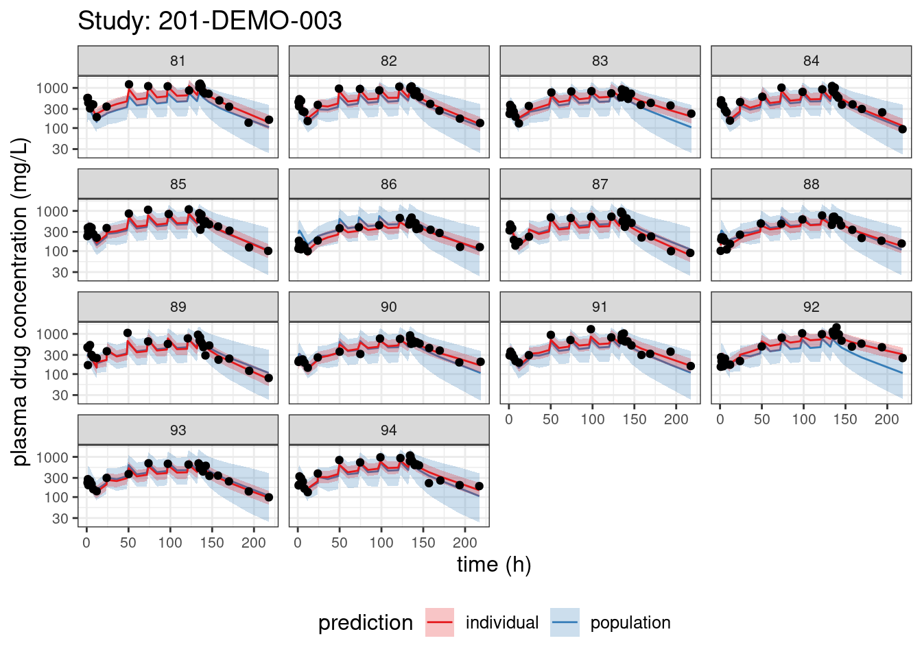
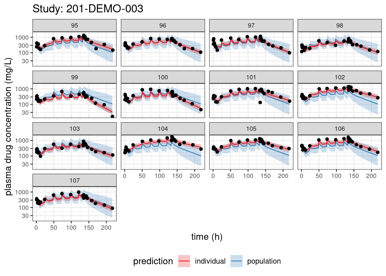
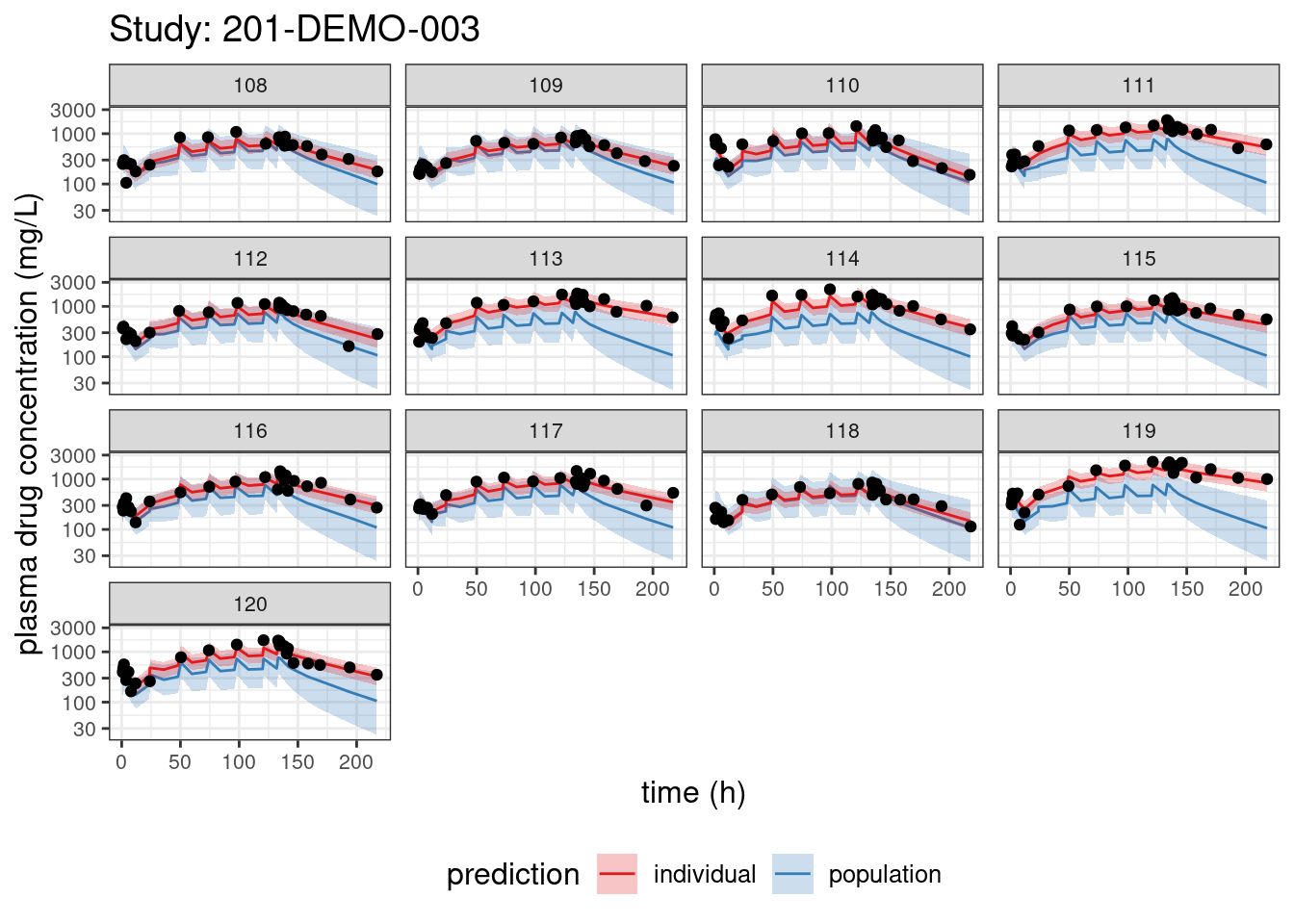
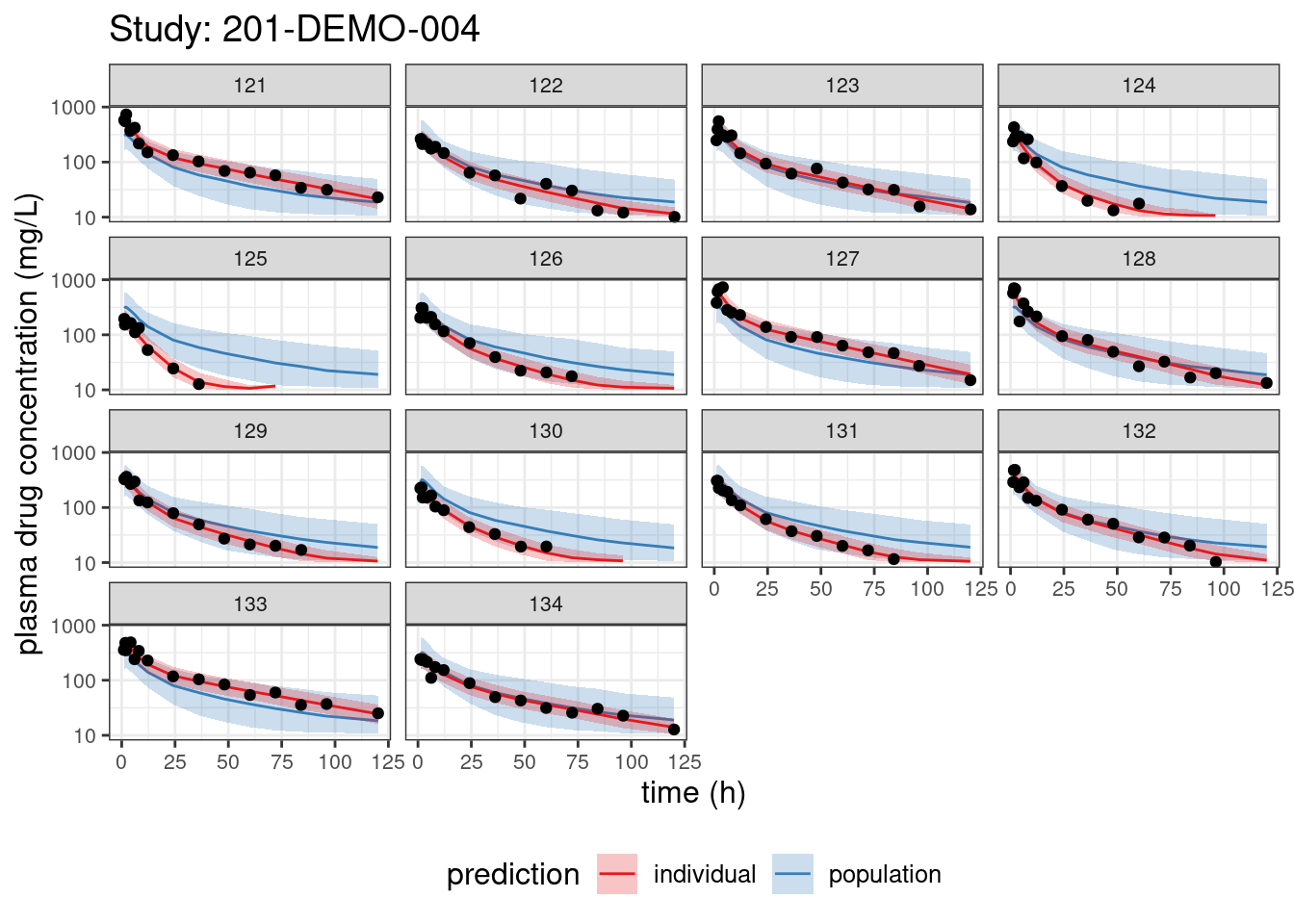
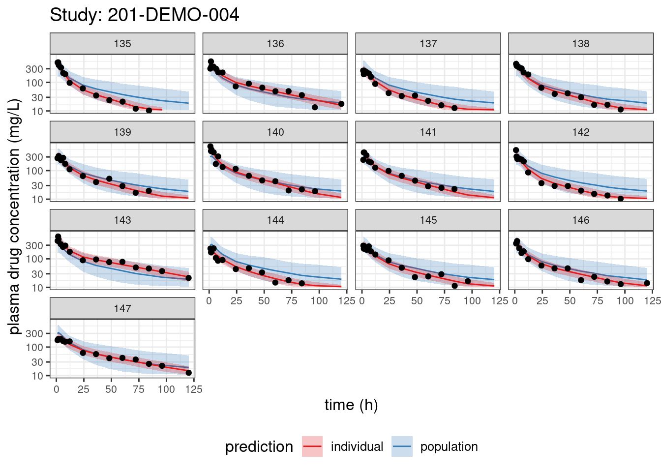
Figure 1: Posterior predictive check for each individual using model ppkexpo1.

Figure 2: Posterior predictive check for each individual using model ppkexpo1.

Figure 3: Posterior predictive check for each individual using model ppkexpo1.

Figure 4: Posterior predictive check for each individual using model ppkexpo1.

Figure 5: Posterior predictive check for each individual using model ppkexpo1.

Figure 6: Posterior predictive check for each individual using model ppkexpo1.

Figure 7: Posterior predictive check for each individual using model ppkexpo1.

Figure 8: Posterior predictive check for each individual using model ppkexpo1.

Figure 9: Posterior predictive check for each individual using model ppkexpo1.

Figure 10: Posterior predictive check for each individual using model ppkexpo1.

Figure 11: Posterior predictive check for each individual using model ppkexpo1.

Figure 12: Posterior predictive check for each individual using model ppkexpo1.

PPCs for each study

PPCs comparing the posterior distributions of landmark statistics (e.g., percentiles like the median and the 5th and 95th percentiles), with the corresponding statistics for the observed data, provide a better assessment of the overall predictive performance of the model. The following code generates such PPCs for each or the four studies in our dataset.

pred2 <- spread_draws(fit, 
                     cPredNew[num]) %>%
  mutate(cPredNew = ifelse(cPredNew < loq, NA_real_, cPredNew)) %>%
  left_join(data2 %>% mutate(num = 1:n())) %>%
  mutate(cPredNew = ifelse(EVID == 1 | TIME == 0, NA_real_, cPredNew))

ppc_all <- observed(data2, x = TIME, y = DV) %>%
  simulated(pred2 %>% arrange(.draw, num), y = cPredNew) %>% 
  stratify(~ STUDY) %>% 
  binning(bin = 'jenks', nbins = 10) %>% 
  vpcstats()

plot(ppc_all, legend.position = "top", 
     color = c("steelblue3", "grey60", "steelblue3"),
     linetype = c("dashed", "solid", "dashed"),
     ribbon.alpha = 0.5) + 
  scale_y_log10() +
  labs(x = "time (h)",
       y = "plasma drug concentration (mg/L)")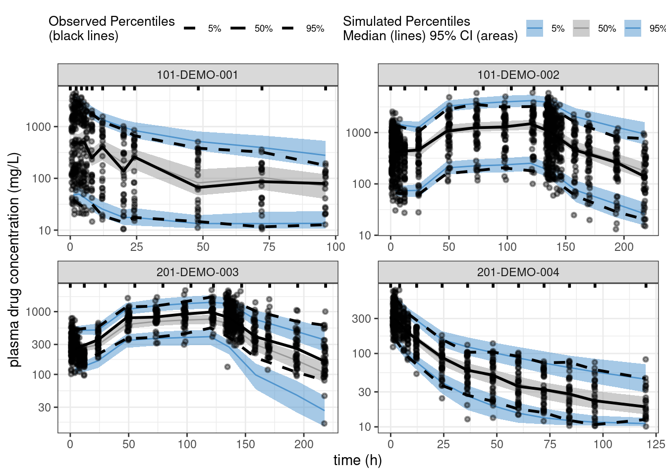

Figure 13: Posterior predictive check for model ppkexpo1.

PPCs for fraction of BLQs

This is a predictive check of the fraction of observations that are below the limit of quantification (BLQ) versus time. We take just the single dose studies and limit the analysis out to 100 hours after the dose.

pred3 <- spread_draws(fit, 
                     cPredNew[num]) %>%
  left_join(data2 %>% mutate(num = 1:n())) %>%
  mutate(BLQsim = ifelse(cPredNew < loq, 1, 0),
         BLQsim = ifelse(EVID == 0, BLQsim, NA_integer_)) %>% 
  filter(STUDY %in% c("101-DEMO-001", "201-DEMO-004"),
         TIME <= 100)

data3 <- data2 %>%
  filter(STUDY %in% c("101-DEMO-001", "201-DEMO-004"),
         TIME <= 100)

ppc_blq <- observed(data3, x = TIME, y = BLQ) %>%
  simulated(pred3 %>% arrange(.draw, num), y = BLQsim) %>% 
  stratify(~ STUDY) %>% 
  binning(bin = 'jenks', nbins = 10) %>% 
  vpcstats(vpc.type = "categorical")

## Change factor labels to make more readable
ppc_blq$stats <- ppc_blq$stats %>%
  mutate(pname = factor(pname, labels = c(">= LOQ", "< LOQ")))

plot(ppc_blq, legend.position = "top",
     ribbon.alpha = 0.5,
     xlab = "time (h)",
     ylab = "fraction above or below LOQ")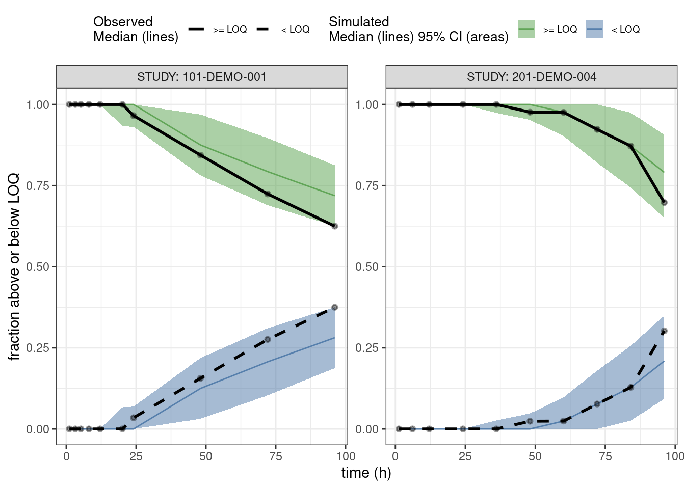

Figure 14: Posterior predictive check of the the fraction of observations that are BLQ for model ppkexpo1.

Other resources

The following script from the GitHub repository is discussed on this page. If you’re interested running this code, visit the About the GitHub Repo page first.

Model Diagnostics script: model-diagnostics.Rmd