library(bbr)
library(bbr.bayes)
library(here)
library(tidyverse)
library(posterior)
library(bayesplot)
library(glue)
library(kableExtra)

cmdstanr::set_cmdstan_path(path = here("Torsten", "v0.91.0", "cmdstan"))

source(here("script", "mcmc-diagnostic-functions.R"))

MODEL_DIR <- here("model", "stan")

bayesplot::color_scheme_set('viridis')
theme_set(theme_bw())Introduction
In this Expo, we make the distinction between two types of diagnostics:
- Markov Chain Monte Carlo (MCMC) convergence diagnostics
- Model diagnostics, aka, goodness-of-fit (GOF) diagnostics
This page demonstrates the use of bbr.bayes, and other tools, to generate MCMC diagnostics for Stan/Torsten Bayesian (Bayes) models.
There is no explicit functionality in bbr.bayes to perform these steps; however, the output from bbr.bayes makes these steps relatively simple.
Tools used
MetrumRG packages
bbr Manage, track, and report modeling activities, through simple R objects, with a user-friendly interface between R and NONMEM®.
bbr.bayes Extension of the bbr package to support Bayesian modeling with Stan or NONMEM®.
CRAN packages
dplyr A grammar of data manipulation.
bayesplot Plotting Bayesian models and diagnostics with ggplot.
posterior Provides tools for working with output from Bayesian models, including output from CmdStan.
Set up
Load required packages and set file paths to your model and figure directories.
MCMC diagnostics
After fitting the model, we examine a suite of MCMC diagnostics to see if anything is amiss with the sampling. Focus on split Rhat, bulk and tail ESS (effective sample size), trace plots, and density plots. If any of these raise a flag about convergence, then additional diagnostics would be examined.
Model summary
We begin by reading in the output from our first base model, ppkexpo1. This is done using the read_fit_model function from bbr.bayes which returns a CmdStanMCMC object that provides several methods for querying the fitting results. For example, fit$draws() returns a draws array containing the MCMC samples.
model_name <- "ppkexpo1"
mod <- read_model(here(MODEL_DIR, model_name))
fit <- read_fit_model(mod)

fit$cmdstan_diagnose()
. Processing csv files: /data/expos/expo4-torsten-poppk/model/stan/ppkexpo1/ppkexpo1-output/ppkexpo1-202409271413-1-0c80d9.csv, /data/expos/expo4-torsten-poppk/model/stan/ppkexpo1/ppkexpo1-output/ppkexpo1-202409271413-2-0c80d9.csv, /data/expos/expo4-torsten-poppk/model/stan/ppkexpo1/ppkexpo1-output/ppkexpo1-202409271413-3-0c80d9.csv, /data/expos/expo4-torsten-poppk/model/stan/ppkexpo1/ppkexpo1-output/ppkexpo1-202409271413-4-0c80d9.csv
.
. Checking sampler transitions treedepth.
. Treedepth satisfactory for all transitions.
.
. Checking sampler transitions for divergences.
. No divergent transitions found.
.
. Checking E-BFMI - sampler transitions HMC potential energy.
. The E-BFMI, 0.09, is below the nominal threshold of 0.30 which suggests that HMC may have trouble exploring the target distribution.
. If possible, try to reparameterize the model.
.
. Effective sample size satisfactory.
.
. The following parameters had split R-hat greater than 1.05:
. omega[2], omega[4], theta[138,2], Q[138], Omega[2,2], Omega[4,2], Omega[2,4], Omega[4,4]
. Such high values indicate incomplete mixing and biased estimation.
. You should consider regularizating your model with additional prior information or a more effective parameterization.
.
. Processing complete.pars <- c("CLHat", "QHat", "V2Hat", "V3Hat", "kaHat",
"sigma", glue("omega[{1:5}]"),
paste0("rho[", matrix(apply(expand.grid(1:5, 1:5),
1, paste, collapse = ","),
ncol = 5)[upper.tri(diag(5),
diag = FALSE)], "]"))
# Get posterior samples for parameters of interest
posterior <- fit$draws(variables = pars)
# Get quantities related to NUTS performance, e.g., occurrence of
# divergent transitions
np <- nuts_params(fit)
n_iter <- dim(posterior)[1]
n_chains <- dim(posterior)[2]
draws_sum <- fit$summary(variables = pars)
ptable <- draws_sum %>%
mutate(across(-variable, ~ pmtables::sig(.x, maxex = 4))) %>%
rename(parameter = variable) %>%
mutate("90% CI" = paste("(", q5, ", ", q95, ")",
sep = "")) %>%
select(parameter, mean, median, sd, mad, "90% CI", ess_bulk, ess_tail, rhat)
ptable %>%
kable %>%
kable_styling()| parameter | mean | median | sd | mad | 90% CI | ess_bulk | ess_tail | rhat |
|---|---|---|---|---|---|---|---|---|
| CLHat | 3.11 | 3.11 | 0.113 | 0.109 | (2.93, 3.30) | 2460 | 1570 | 1.00 |
| QHat | 3.80 | 3.80 | 0.178 | 0.187 | (3.52, 4.09) | 118 | 192 | 1.02 |
| V2Hat | 60.9 | 60.8 | 2.23 | 2.24 | (57.3, 64.6) | 278 | 494 | 1.00 |
| V3Hat | 67.7 | 67.7 | 1.87 | 1.90 | (64.7, 70.8) | 334 | 990 | 1.00 |
| kaHat | 1.61 | 1.60 | 0.117 | 0.116 | (1.43, 1.82) | 340 | 778 | 1.00 |
| sigma | 0.214 | 0.214 | 0.00304 | 0.00297 | (0.208, 0.219) | 2000 | 1600 | 1.00 |
| omega[1] | 0.436 | 0.435 | 0.0250 | 0.0254 | (0.397, 0.479) | 2380 | 1620 | 1.00 |
| omega[2] | 0.131 | 0.123 | 0.0609 | 0.0657 | (0.0406, 0.234) | 18.8 | 42.1 | 1.17 |
| omega[3] | 0.377 | 0.376 | 0.0266 | 0.0283 | (0.335, 0.421) | 412 | 1200 | 1.01 |
| omega[4] | 0.182 | 0.182 | 0.0291 | 0.0288 | (0.135, 0.231) | 66.6 | 413 | 1.05 |
| omega[5] | 0.545 | 0.543 | 0.0709 | 0.0713 | (0.433, 0.667) | 183 | 470 | 1.01 |
| rho[1,2] | -0.132 | -0.152 | 0.268 | 0.270 | (-0.549, 0.339) | 184 | 381 | 1.02 |
| rho[1,3] | 0.676 | 0.680 | 0.0604 | 0.0607 | (0.576, 0.771) | 172 | 572 | 1.02 |
| rho[2,3] | 0.0912 | 0.0820 | 0.275 | 0.299 | (-0.349, 0.547) | 168 | 383 | 1.02 |
| rho[1,4] | 0.332 | 0.337 | 0.137 | 0.136 | (0.0958, 0.543) | 348 | 787 | 1.01 |
| rho[2,4] | 0.366 | 0.409 | 0.268 | 0.274 | (-0.122, 0.748) | 126 | 325 | 1.04 |
| rho[3,4] | 0.546 | 0.552 | 0.154 | 0.162 | (0.286, 0.793) | 113 | 148 | 1.03 |
| rho[1,5] | 0.600 | 0.607 | 0.0880 | 0.0911 | (0.451, 0.737) | 486 | 863 | 1.01 |
| rho[2,5] | -0.387 | -0.435 | 0.303 | 0.290 | (-0.820, 0.196) | 81.2 | 191 | 1.04 |
| rho[3,5] | 0.436 | 0.443 | 0.107 | 0.109 | (0.253, 0.593) | 236 | 401 | 1.01 |
| rho[4,5] | -0.103 | -0.111 | 0.196 | 0.203 | (-0.417, 0.220) | 128 | 349 | 1.02 |
For the population-level parameters, the Rhat values are less than or equal to 1.05 except for omega[2]. Also, some ESS bulk and tail values are on the low side. In addition, a couple divergent transitions occurred.
Rhat plot
We visualize the Rhat values with the mcmc_rhat function from bayesplot.
rhats <- draws_sum$rhat
names(rhats) <- draws_sum$variable
rhat_plot <- mcmc_rhat(rhats) + yaxis_text()
rhat_plot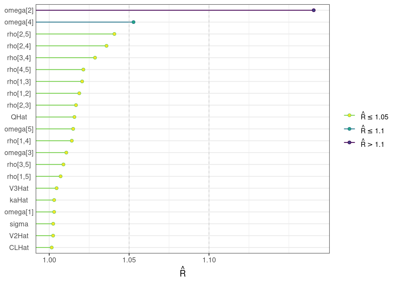
ESS plots
We can also visualize the bulk and tail ESS as ratios of the effective sample size (Neff) to the total number of iterations (N).
ess_bulk <- draws_sum$ess_bulk
names(ess_bulk) <- draws_sum$variable
ess_bulk_ratios <- ess_bulk / (n_iter * n_chains)
ess_bulk_plot <- mcmc_neff(ess_bulk_ratios) + yaxis_text() +
  labs(title = "Bulk ESS ratios")
ess_bulk_plot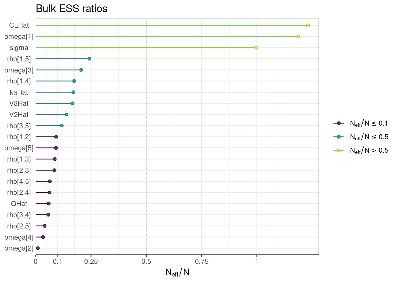
ess_tail <- draws_sum$ess_tail
names(ess_tail) <- draws_sum$variable
ess_tail_ratios <- ess_tail / (n_iter * n_chains)
ess_tail_plot <- mcmc_neff(ess_tail_ratios) + yaxis_text() +
  labs(title = "Tail ESS ratios")
ess_tail_plot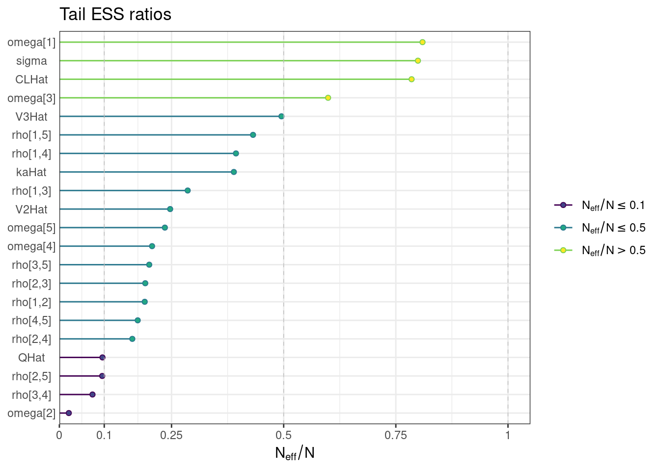
Trace and density plots
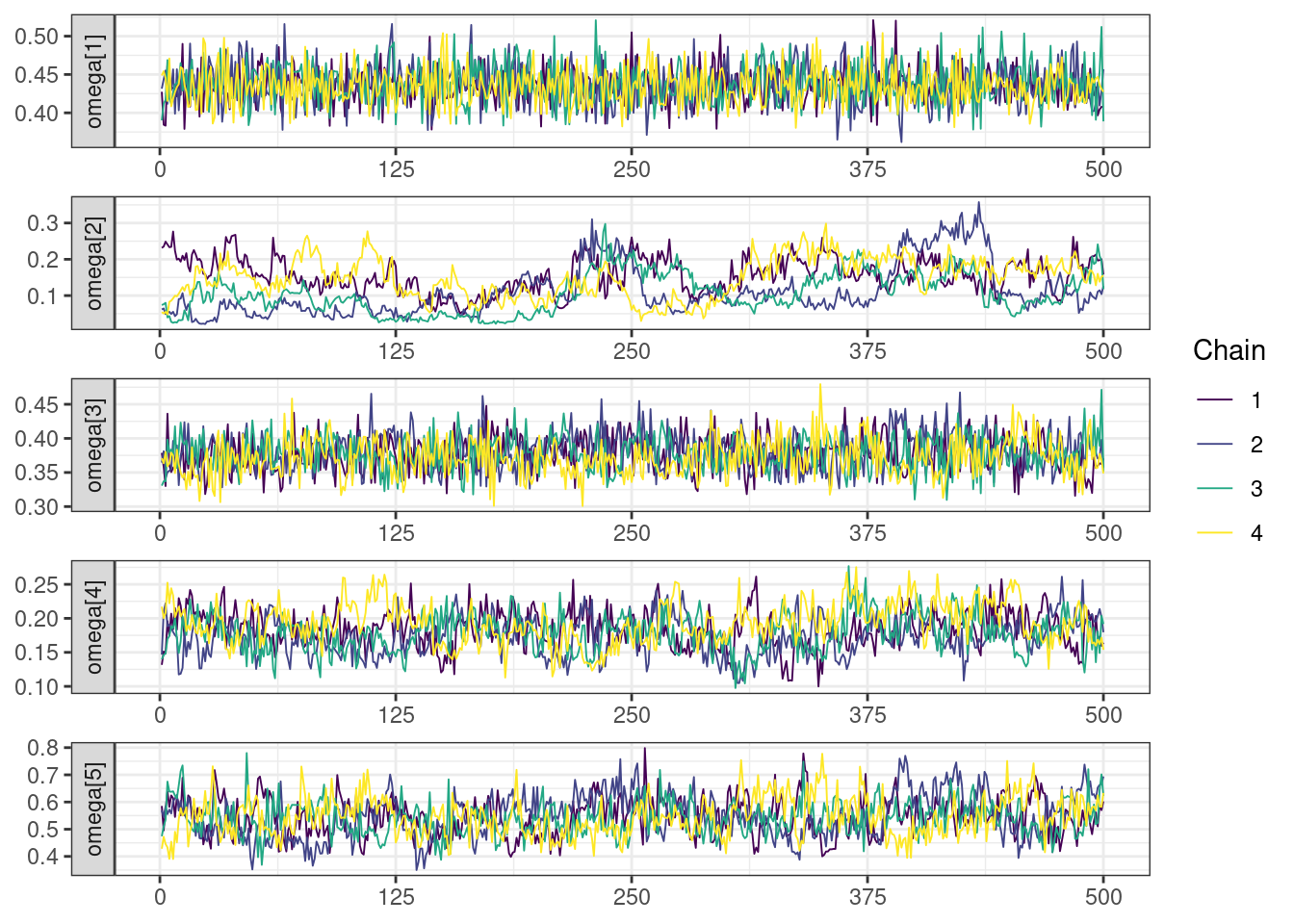
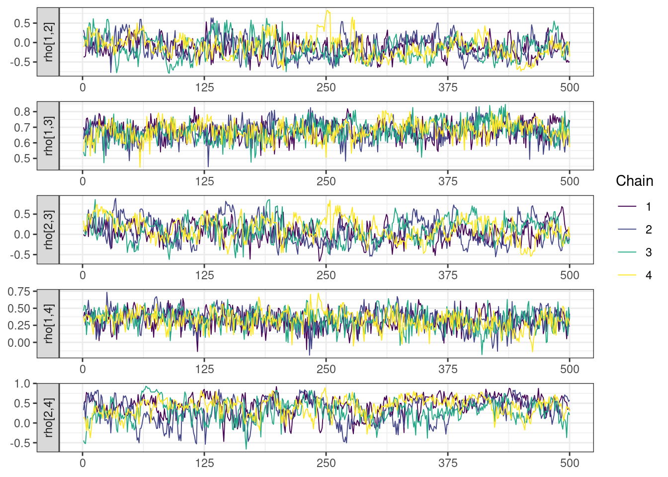
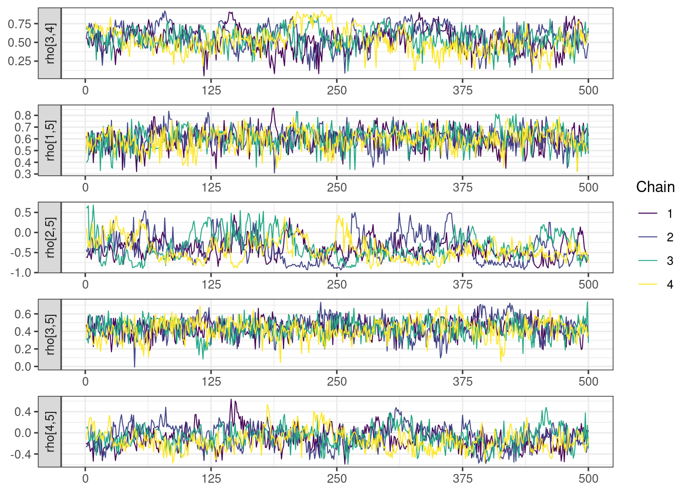
Next, we look at the trace and density plots.
mcmc_history_plots <- mcmc_history(posterior,
                                  nParPerPage = 6,
np = np)mcmc_history_plots. [[1]].
. [[2]].
. [[3]].
. [[4]]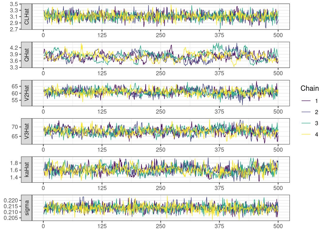
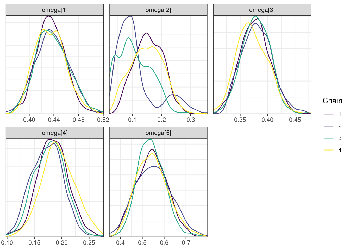
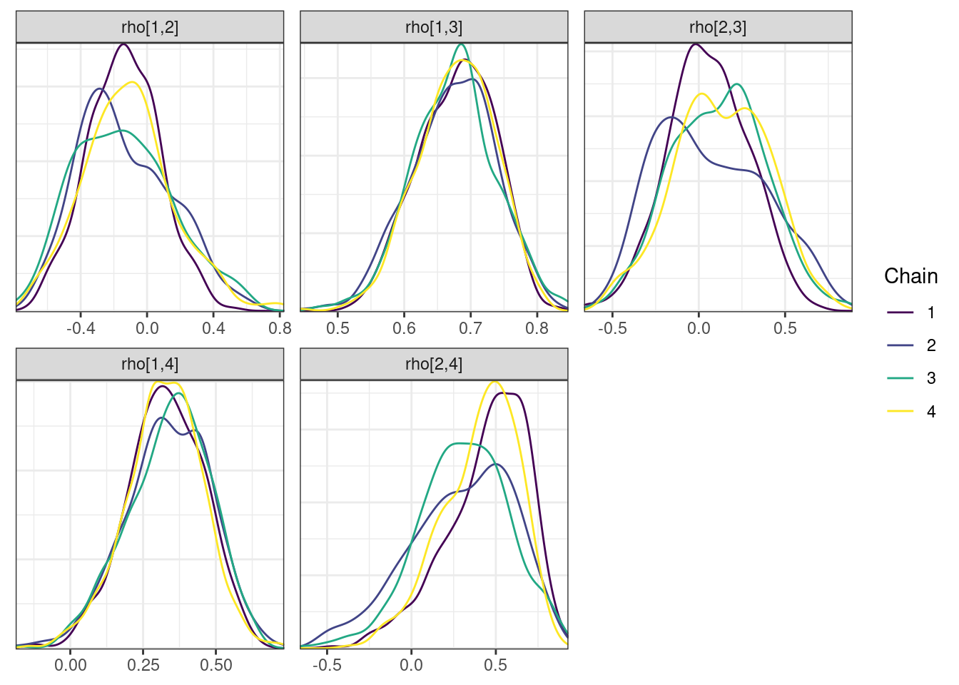
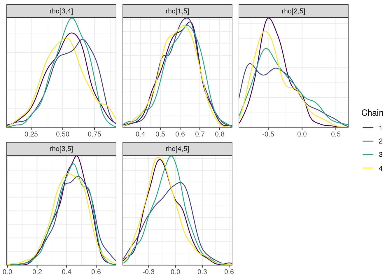
  mcmc_density_chain_plots <- mcmc_density(posterior,
nParPerPage = 6, byChain = TRUE)mcmc_density_chain_plots. [[1]].
. [[2]].
. [[3]].
. [[4]]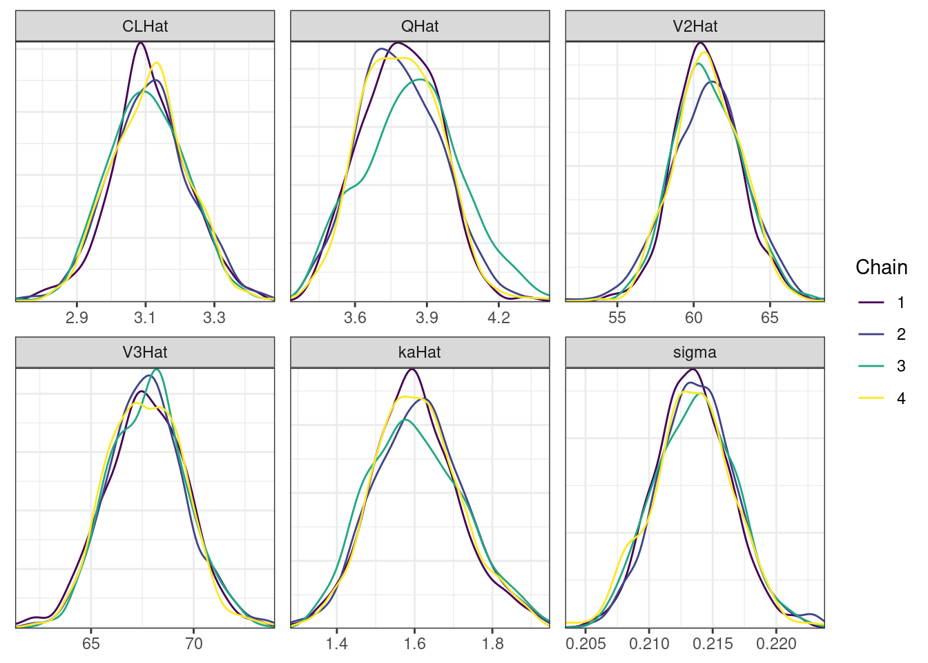
A scatterplot of the MCMC draws can be useful in showing bivariate relationships in the posterior distribution. The default scatterplot generated with mcmc_pairs uses points for the off-diagonal panels and histograms along the diagonal. We restrict this plot to only CLHat, QHat, V2Hat, V3Hat, kaHat, and sigma.
pairs_plot <- mcmc_pairs(posterior, pars = pars[!(grepl("rho", pars) | grepl("omega", pars))])pairs_plot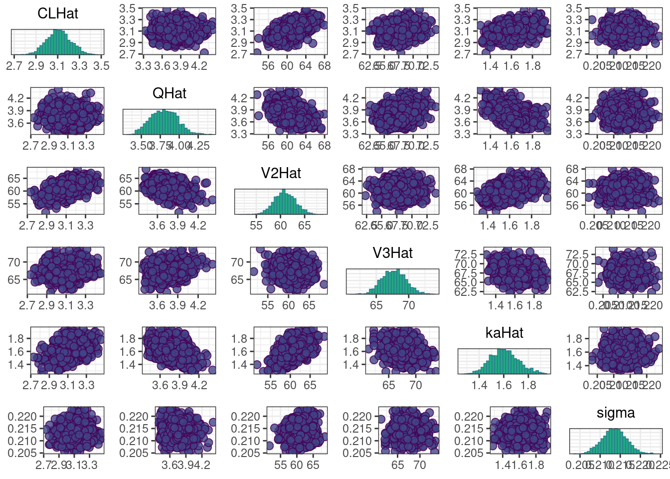
A more informative plot might use density estimates and transformations to bounded parameters. We can make these modifications using the diag_fun, off_diag_fun, and transformations arguments:
pairs_plot2 <- mcmc_pairs(posterior,
           pars = pars[!(grepl("rho", pars) | grepl("omega",
                                                           pars))],
           transformations = "log",
           diag_fun = 'dens',
           off_diag_fun = 'hex')
pairs_plot2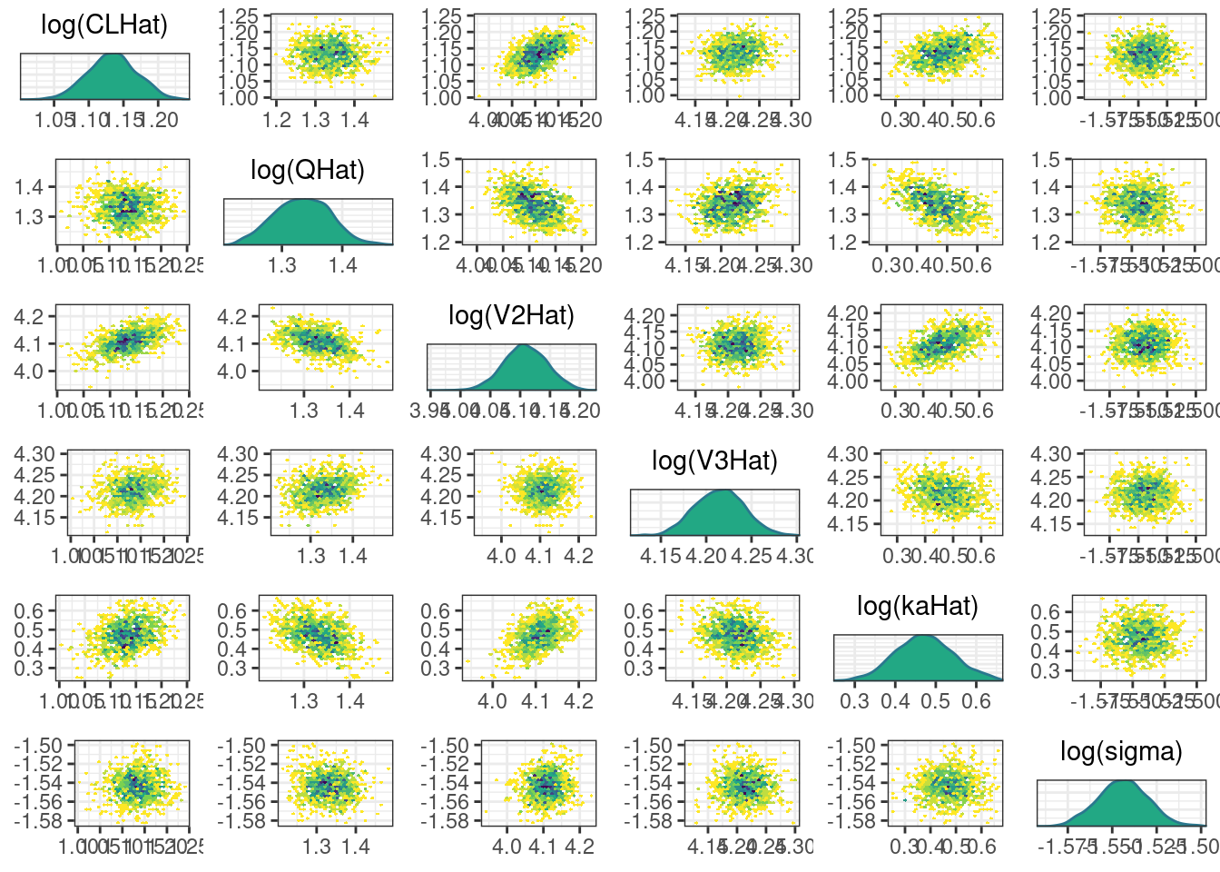
While most MCMC diagnostics look reasonably good, omega[2] is a notable exception as shown by a large Rhat, low effective sample sizes, a “wiggly snake” trace plot, and density plots indicating differences among the chains. The small number of divergent transitions, while not serious, suggests we should consider some intervention. The next logical steps are to increase the number of MCMC iterations, or reparameterize, to improve sampling performance (or both).
Other resources
The following script from the GitHub repository is discussed on this page. If you’re interested running this code, visit the About the GitHub Repo page first.
MCMC Diagnostics script: mcmc-diagnostics.Rmd
More details on the visual MCMC diagnostics are available in a Vignettes from bayesplot package developers.