Introduction

Model summaries provide a condensed overview of the key decisions made during the model development process. They’re quick to compile and take advantage of the easy annotation features of bbr, such as the description, notes, and tags, to summarize the important features of key models.

The page demonstrates how to:

Create and modify model run logs
Check and compare model tags
Graphically represent the relationships between models

For a walk-though on how to define, submit, and annotate your models, see the Fitting Your Initial Model page.

Tools used

MetrumRG packages

bbr Manage, track, and report modeling activities, through simple R objects, with a user-friendly interface between R and NONMEM®.

CRAN packages

dplyr A grammar of data manipulation.

Set up

Load required packages and set file paths to your model and figure directories.

library(bbr)
library(bbr.bayes)
library(dplyr)
library(here)
library(tidyverse)
library(yspec)
library(posterior)
library(igraph)

MODEL_DIR <- here("model", "stan","expo")
FIGURE_DIR <- here("deliv", "figure","expo")

Modeling Summary

We can also create a run log of all, or a subset, of the models we’ve fit:

log_df <- run_log(MODEL_DIR) %>%
  collapse_to_string(based_on)

The return object is a tibble with information about each model, including where the model resides on disk; the model type (stan vs stan_gq); model description, tags and notes added to the model object; and a field indicating the model on which each model is based. For our worked example, a glimpse of log_df looks like this:

glimpse(log_df)

. Rows: 11
. Columns: 10
. $ absolute_model_path <chr> "/data/expo2-stan/model/stan/expo/mod0", "/data/ex…
. $ run                 <chr> "mod0", "mod0_gq", "mod0a", "mod1", "mod1_gq", "mo…
. $ yaml_md5            <chr> "d17890ab3d36b245224efe614f7ea981", "ae4ac7ef5a74f…
. $ model_type          <chr> "stan", "stan_gq", "stan", "stan", "stan_gq", "sta…
. $ description         <chr> "Base model with non-centered parameterization.", …
. $ bbi_args            <list> <NULL>, <NULL>, <NULL>, <NULL>, <NULL>, <NULL>, <…
. $ based_on            <chr> NA, "mod0", "mod0", "mod0", "mod1", "mod1", "mod1"…
. $ tags                <list> <"non-centered parameterization", "4 Parameter (s…
. $ notes               <list> <"Sigmoidal Emax function of dose.  No covariates…
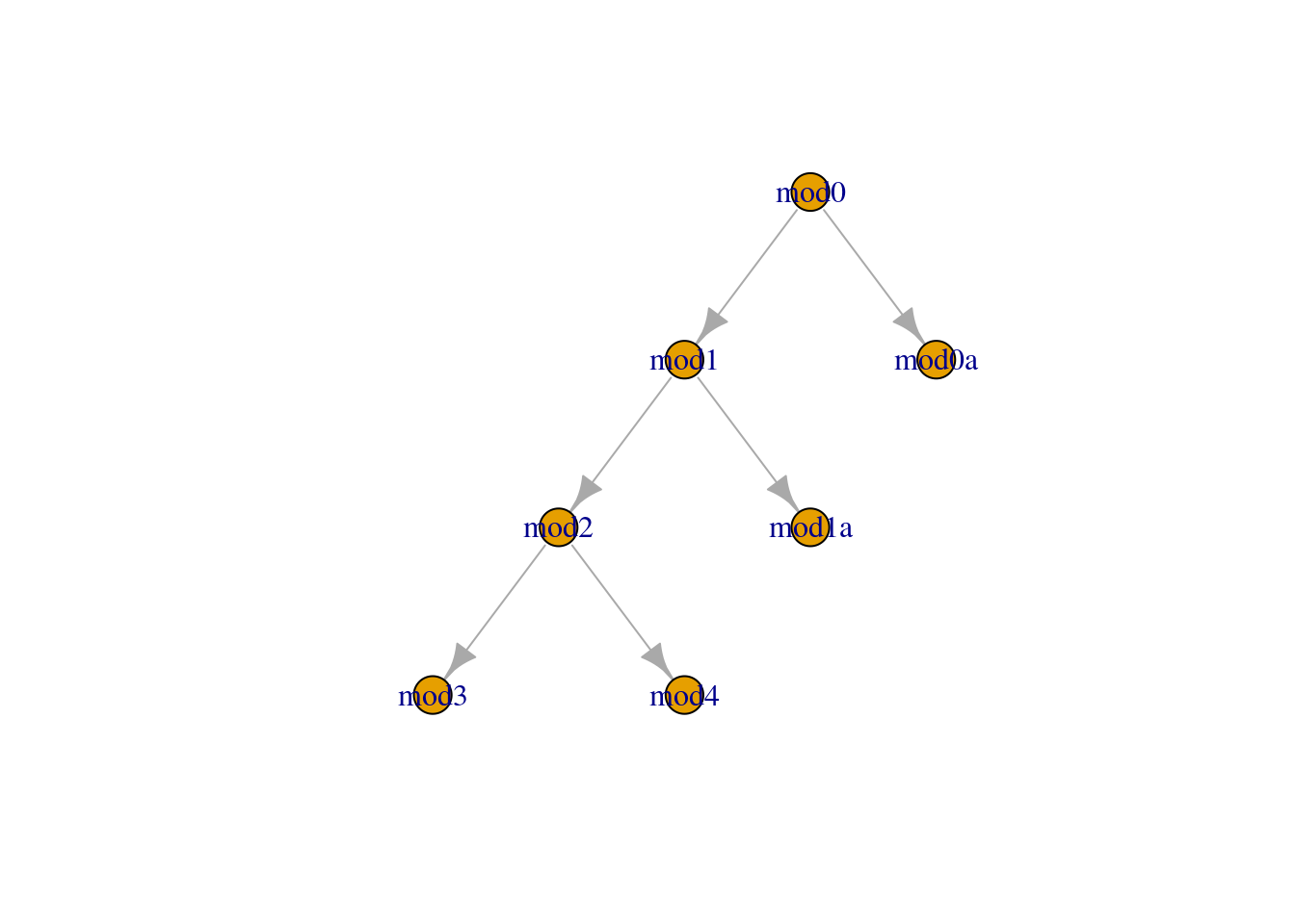
. $ star                <lgl> FALSE, FALSE, FALSE, FALSE, FALSE, FALSE, FALSE, F…

We can graphically represent the relationships between our models by plotting the network:

log_df_subset <- log_df %>%
  filter(model_type=='stan') %>% 
  filter(based_on!='') %>% 
  select(from=based_on, to=run)

model_graph <- graph_from_data_frame(log_df_subset)

plot(model_graph,layout=layout_as_tree)

run_log() provides qualitative information about each model to give an overview of the modeling process. We can also extract some quantiative measures of model fit and NUTS diagnostics using the stan_summary_log function instead of run_log. That collects Stan models from the specified directory and returns a dedicated tibble; alternatively, you can add this information to a run log using stan_add_summary.

log_df_quant <- log_df %>%
  filter(model_type == 'stan') %>% 
  stan_add_summary()

By default, the resulting tibble contains the following fields, in addition to those in the run_log object:

. Rows: 7
. Columns: 15
. $ method            <chr> "sample", "sample", "sample", "sample", "sample", "s…
. $ stan_version      <chr> "2.33.0", "2.33.0", "2.33.0", "2.33.0", "2.33.0", "2…
. $ nchains           <int> 4, 4, 4, 4, 4, 4, 4
. $ iter_warmup       <int> 1000, 1000, 1000, 1000, 1000, 1000, 1000
. $ iter_sampling     <int> 1000, 1000, 1000, 1000, 1000, 1000, 1000
. $ num_divergent     <int> 1, 42, 0, 28, 0, 0, 0
. $ num_max_treedepth <int> 0, 0, 0, 52, 0, 0, 0
. $ bad_ebfmi         <lgl> FALSE, TRUE, TRUE, TRUE, FALSE, FALSE, FALSE
. $ lp___mean         <dbl> -3340.057, -3239.543, -3217.506, -3202.821, -3339.96…
. $ lp___median       <dbl> -3339.885, -3243.845, -3226.175, -3214.770, -3339.26…
. $ lp___q5           <dbl> -3358.100, -3294.890, -3295.750, -3284.773, -3358.90…
. $ lp___q95          <dbl> -3323.278, -3172.950, -3105.970, -3083.180, -3322.45…
. $ lp___rhat         <dbl> 1.002087, 1.035124, 1.070815, 1.358419, 1.001309, 1.…
. $ lp___ess_bulk     <dbl> 1052.919360, 84.383630, 34.610611, 9.482857, 1091.03…
. $ lp___ess_tail     <dbl> 2021.74820, 167.40749, 70.74767, 23.14587, 1889.1205…

Additional variables can be added using the variables and summary_fns arguments. For example, if we wanted to add the posterior mean and Monte Carlo standard error for emax, tv_ec50 and lp__, we would use the following:

log_df_quant2 <- log_df %>%
  filter(model_type == 'stan') %>% 
  stan_add_summary(variables = c('emax','tv_ec50',
                                 'lp__'),
                   summary_fns = list('mean','mcse_mean',
                                      'rhat'))

The resulting tibble now contains the following variables:

. Rows: 7
. Columns: 17
. $ method            <chr> "sample", "sample", "sample", "sample", "sample", "s…
. $ stan_version      <chr> "2.33.0", "2.33.0", "2.33.0", "2.33.0", "2.33.0", "2…
. $ nchains           <int> 4, 4, 4, 4, 4, 4, 4
. $ iter_warmup       <int> 1000, 1000, 1000, 1000, 1000, 1000, 1000
. $ iter_sampling     <int> 1000, 1000, 1000, 1000, 1000, 1000, 1000
. $ num_divergent     <int> 1, 42, 0, 28, 0, 0, 0
. $ num_max_treedepth <int> 0, 0, 0, 52, 0, 0, 0
. $ bad_ebfmi         <lgl> FALSE, TRUE, TRUE, TRUE, FALSE, FALSE, FALSE
. $ emax_mean         <dbl> 98.57265, 98.64793, 98.58554, 98.54141, 98.61974, 98…
. $ tv_ec50_mean      <dbl> 97.33520, 97.58208, 97.47109, 97.50115, 97.65860, 98…
. $ lp___mean         <dbl> -3340.057, -3239.543, -3217.506, -3202.821, -3339.96…
. $ emax_mcse_mean    <dbl> 0.01888614, 0.03496757, 0.02004958, 0.03730079, 0.01…
. $ tv_ec50_mcse_mean <dbl> 0.08178114, 0.16565652, 0.08966909, 0.20720041, 0.09…
. $ lp___mcse_mean    <dbl> 0.3281358, 4.1744750, 9.9832907, 21.5147029, 0.33146…
. $ emax_rhat         <dbl> 0.9997144, 1.0036807, 1.0008757, 1.0019203, 1.002241…
. $ tv_ec50_rhat      <dbl> 1.000972, 1.004725, 1.000948, 1.002428, 1.003337, 1.…
. $ lp___rhat         <dbl> 1.002087, 1.035124, 1.070815, 1.358419, 1.001309, 1.…

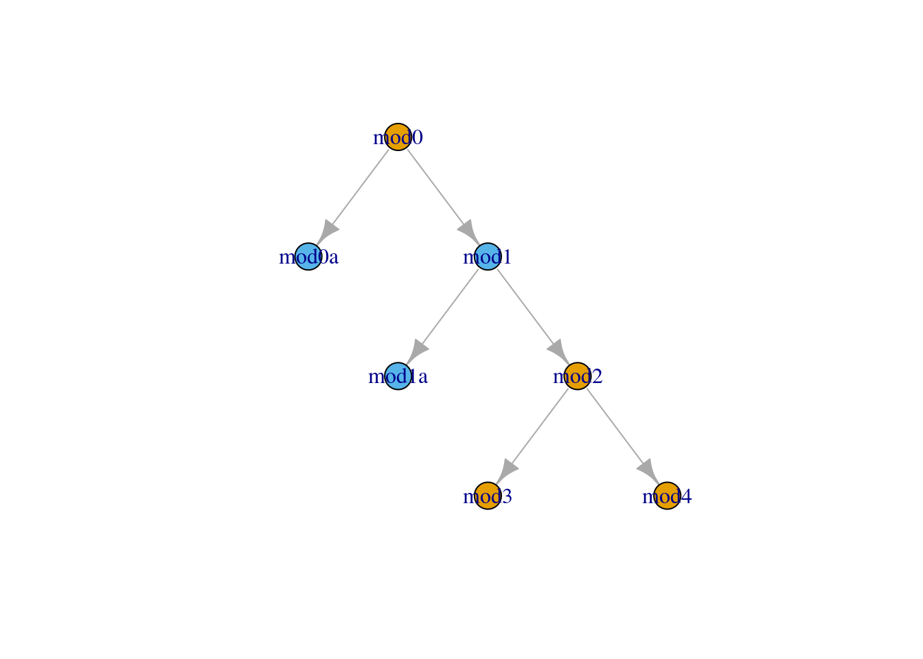
We can use information from the run log or run summary to enhance the graphical representation of the model. For example, we might want to highlight models which have a high Rhat value for the log posterior value:

subset_to_plot <- log_df_quant2 %>%
  filter(model_type=='stan') %>% 
  filter(based_on!='') %>% 
  select(from=based_on, to=run)

vertex_data <- log_df_quant2 %>%
  filter(model_type=='stan')  %>% 
  select(run,bad_ebfmi,lp___rhat) %>% 
  mutate(`High Rhat` = as.numeric(lp___rhat > 1.01)+1)

model_graph <- graph_from_data_frame(subset_to_plot ,
                                     vertices = vertex_data)
V(model_graph)$color <- categorical_pal(2)[vertex_data$`High Rhat`]

plot(model_graph,layout=layout_as_tree)

Graphical relationship of models. Blue nodes represent models with Rhat > 1.01 for the log posterior.

Other resources

The following script from the GitHub repository is discussed on this page. If you’re interested running this code, visit the About the GitHub Repo page first.

Modeling Summary script: modeling-summary.Rmd