Introduction

Managing the model development process in a traceable and reproducible manner can be a significant challenge. At MetrumRG, we use bbr and bbr.bayes to streamline this process for fitting Bayesian models. This Expo will demonstrate an example workflow for fitting models using Stan.

bbr and bbr.bayes are R packages developed by MetrumRG that serve three primary purposes:

Submit models, particularly for execution in parallel and/or on a high-performance compute (HPC) cluster (e.g. Metworx).
Parse model outputs into R objects to facilitate model evaluation and diagnostics in R.
Annotate the model development process for easy and reliable traceability and reproducibility.

This page demonstrates the following bbr and bbr.bayes functionality:

Creating and submitting an initial model

Tools used

MetrumRG packages

bbr Manage, track, and report modeling activities, through simple R objects, with a user-friendly interface between R and NONMEM®.

bbr.bayes Extension of the bbr package to support Bayesian modeling with Stan or NONMEM®

CRAN packages

dplyr A grammar of data manipulation.

Outline

This page details a range of tasks frequently performed throughout the modeling process such as defining, submitting, and annotating models. Typically, our scientists run this code in a scratch pad style script, since it isn’t necessary for the entire coding history for each model to persist. Here, the code used each step of the process is provided as a reference, and a runnable version of this page is available in our GitHub repository: initial-model-submission.Rmd.

If you’re a new bbr user, we recommend you read through the Getting Started vignette before trying to run any code. This vignette includes some setup and configuration requirement (e.g., making sure bbr can find your cmdstan installation).

Please note that bbr doesn’t edit the model structure in your Stan code. This page walks through a sequence of models that might evolve during a simple modeling project. All modifications to the Stan code are made directly by the modeler. Below, we’ve included comments asking you to edit your Stan code manually.

After working through this content, we recommend reading the Model Summary page and accompanying modeling-summary.Rmd file. The purpose of the modeling-summary.Rmd is to provide a high-level overview of the project’s current status. Also, we show how to leverage the model annotation to summarize your modeling work, specifically, how to create model run logs using bbr::run_log() and bbr.bayes::stan_add_summary() to summarize key features of each model (including the descriptions, notes, and tag fields) and provide suggestions for model notes that capture key decision points in the modeling process.

Set up

Load required packages and set file paths to your model and figure directories.

library(bbr)
library(bbr.bayes)
library(dplyr)
library(here)
library(tidyverse)
library(yspec)
library(tidyvpc)
library(bayesplot)
library(loo)

MODEL_DIR <- here("model", "stan","expo")
FIGURE_DIR <- here("deliv", "figure","expo")

Model creation and submission

Initial Stan model file

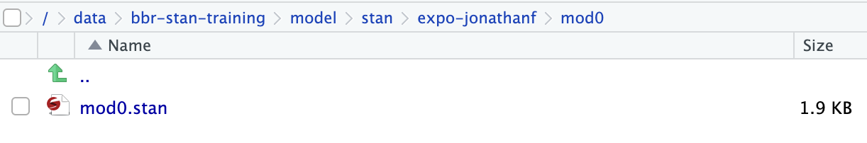
Before using bbr, you’ll need to have a Stan model file describing your first model. We’ll name our first model file mod0.stan. Note that this initial model must be saved in whatever location is defined as MODEL_DIR and additionally embedded within a subdirectory with the same name as the stan model, mod0 in this case. In the typical MRG file structure used here, MODEL_DIR is model/stan/, meaning the full path to the initial model is model/stan/mod0/.

The Stan code below implements a non-centered version of this model and includes a generated quantities block to simulate data for posterior predictive checks.


data {
  int<lower=0> N ;
  int<lower=0> n_id ;
  vector[N] DV;
  vector[N] Conc;
  array[N] int ID;
  array[n_id] int start;
  array[n_id] int end;
}

parameters {
  real<lower=0, upper=100> emax;
  real tv_log_ec50;
  real tv_e0;
  real log_gamma;
  
  vector[n_id] eta_log_ec50;
  vector[n_id] eta_e0;
  
  real<lower=0> sigma;
  real<lower=0> omega_e0;
  real<lower=0> omega_log_ec50;
}

transformed parameters {
  real tv_ec50 = exp(tv_log_ec50);
  real gamma = exp(log_gamma);
  vector[n_id] ec50;
  vector[n_id] e0;
  vector[N] mu;
  
  ec50 = exp(tv_log_ec50 + omega_log_ec50 * eta_log_ec50);
  e0 = tv_e0 + omega_e0 * eta_e0;
  
  for (i in 1:N) {
    mu[i] = e0[ID[i]] + (emax-e0[ID[i]])*pow(Conc[i]/100,gamma) / 
               (pow(ec50[ID[i]]/100,gamma) + pow(Conc[i]/100,gamma));
  }
  
}

model {
  // Priors
  tv_e0 ~ normal(0, 10);
  tv_log_ec50 ~ normal(4,2);
  emax ~ uniform(0,100);
  log_gamma ~ normal(0,1);
  sigma ~ normal(0,10);
  omega_e0 ~ normal(0,2);
  omega_log_ec50 ~ normal(0,1);

  eta_e0 ~ std_normal();
  eta_log_ec50 ~ std_normal();

// Likelihhood

  DV ~ normal(mu, sigma);

}

generated quantities {
  vector[N] simdv_obs;
  vector[N] simdv_new;

  // Simulated observations for observed subjects
  for (i in 1:N) {
    simdv_obs[i] = normal_rng(mu[i],sigma);
  }
  
  // Simulate observations for new subject
  {
    vector[n_id] ec50_new;
    vector[n_id] e0_new;
    vector[N] mu_new;
    
    for (i in 1:n_id) {
        ec50_new[i] = lognormal_rng(tv_log_ec50,omega_log_ec50);
        e0_new[i] = normal_rng(tv_e0 , omega_e0);
    }
    
    for (i in 1:N) {
      mu_new[i] = e0_new[ID[i]] + (emax-e0_new[ID[i]])*pow(Conc[i]/100,gamma) / 
                            (pow(ec50_new[ID[i]]/100,gamma) + pow(Conc[i]/100,gamma));
      simdv_new[i] = normal_rng(mu_new[i] , sigma);
    }
  }
  
}

Create a model object

After creating your initial Stan model file, the first step in using bbr.bayes is to create a model object. This model object is passed to all of the other bbr functions that submit, summarize, or manipulate models. You can read more about the model object and the function that creates it, bbr::new_model(), in the Create model object section of the “Getting Started” vignette.

Let’s create our first model object. Note that for Stan models we need to include the .model_type='stan' argument:

Warning: overwrite

Use caution when using the .overwrite= TRUE argument in new_model and copy_model_from. It will overwrite existing files and output directory, if they exist.

mod0 <- new_model(file.path(MODEL_DIR, 'mod0'), 
                  .model_type = 'stan',
                  .overwrite = TRUE)

The first argument to new_model() is the path to your model Stan model file without the file extension. The call above assumes you have a Stan model file mod0.stan in the MODEL_DIR/mod0 directory.

Prior to creating your model object with new_model(), your model directory had one directory (mod0) with one file (mod0/mod0.stan).

The new_model() function creates the set of files necessary for running a Stan model using bbr.bayes. First, the mod0.yaml file is created in your model directory; this file automatically persists any tags, notes, and other model metadata. While it’s useful to know that this YAML file exists, you shouldn’t need to interact with it directly (e.g., in the RStudio file tabs). Instead, bbr has a variety of functions (i.e., add_tags() and add_notes() shown below) that work with the model object to edit the information in the YAML file from your R console.

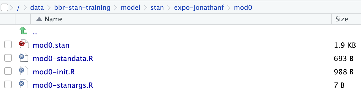
Second, templates for the mod0-standata.R, mod0-init.R, and mod0-stanargs.R files are created in the mod0 directory. Additionally, if no <run>.stan file is detected, bbr.bayes will create a template model for you. The roles of these files are likely self-evident from their names, but a bit more information about their inputs and outputs is provided below:

<run>.stan is a file containing the Stan model code.
<run>-standata.R constructs a function returning a Stan-ready data object which is then passed to the CmdStanModel$sample() call. You can use the build_data() function to view the data object created by the function.
<run>-stanargs.R constructs a named list with all of the arguments that will be passed to the CmdStanModel$sample() call. See set_stanargs() for details on modifying.
<run>-init.R is a file which contains all necessary R code to create the initial values passed to the CmdStanModel$sample() call.

Customizing the model object files

We can interact with each of these files using the associated open_<filetype>_file function.

First, let’s edit the mod0-standata.R file. Recall, the source data file (exdata3.csv) looks like this:

head(exdata3)

. # A tibble: 6 × 8
.      ID weight   age   sex  time  dose  cobs fxa.inh
.   <dbl>  <dbl> <dbl> <dbl> <dbl> <dbl> <dbl>   <dbl>
. 1     1     59    30     1 0      1.25  0       2.78
. 2     1     59    30     1 0.083  1.25  6.19   15.2 
. 3     1     59    30     1 0.167  1.25 13.2     9.16
. 4     1     59    30     1 0.25   1.25 15.3    13.7 
. 5     1     59    30     1 0.5    1.25 22.3    21.5 
. 6     1     59    30     1 0.75   1.25 21.4    37.2

spec <- load_spec(here('data','derived','exdata3.yml'))
exdata3 <- ys_add_factors(exdata3, spec)
ind_exdata3 <- distinct(exdata3, ID, .keep_all = TRUE)

labs <- ys_get_short_unit(spec)

To edit the mod0-standata.R file, we can use the open_standata_file() function:

open_standata_file(mod0)

We manually edit this file to have the contents we want. For this model, the code looks like this:

# Create Stan data
#
# This function must return the list that will be passed to `data` argument
#   of `cmdstanr::sample()`
#
# The `.dir` argument represents the absolute path to the directory containing
#   this file. This is useful for building file paths to the input files you will
#   load. Note: you _don't_ need to pass anything to this argument, you only use
#   it within the function. `bbr` will pass in the correct path when it calls
#   `make_standata()` under the hood.
make_standata <- function(.dir) {
  # read in any input data
  in_data <- readr::read_csv(
    file.path(.dir, "..", "..", "..", "..", "data/derived/exdata3.csv"),
    show_col_types = FALSE
  )
  
  list(
    N = nrow(in_data),
    n_id = length(unique(in_data$ID)),
    DV = in_data$fxa.inh,
    Conc = in_data$cobs,
    ID = in_data$ID,
    start = in_data %>% mutate(num=1:n()) %>% group_by(ID) %>% slice_head(n=1) %>% pull(num),
    end = in_data %>% mutate(num=1:n()) %>% group_by(ID) %>% slice_tail(n=1) %>% pull(num)
  )
}

This R file must create a function named make_standata() which takes the input to the directory where the file is located and returns a list suitable for use with Stan.

Similarly, we can open the file defining how we want the initial values generated.

open_staninit_file(mod0)

We manually edit this file to have the contents we want. For this model, the code looks like this:

# Create Stan initial values
#
# This function must return something that can be passed to the `init` argument
#   of `cmdstanr::sample()`. There are several options; see `?cmdstanr::sample`
#   for details.
#
# `.data` represents the list returned from `make_standata()` for this model.
#   This is provided in case any of your initial values are dependent on some
#   aspect of the data (e.g. the number of rows).
#
# `.args` represents the list of attached arguments that will be passed through to
#   cmdstanr::sample(). This is provided in case any of your initial values are
#   dependent on any of these arguments (e.g. the number of chains).
#
# Note: you _don't_ need to pass anything to either of these arguments, you only
#   use it within the function. `bbr` will pass in the correct objects when it calls
#   `make_init()` under the hood.
#
make_init <- function(.data, .args) {
  # returning NULL causes cmdstanr::sample() to use the default initial values
  return(
    function() {
      list(tv_e0 = rnorm(1),
           emax = runif(1,90,100),
           tv_log_ec50 = rnorm(1,log(100),1),
           log_gamma = rnorm(1,0,.1),
           eta_e0 = rnorm(.data$n_id),
           eta_log_ec50 = rnorm(.data$n_id),
           omega_e0 = abs(rnorm(1)),
           omega_log_ec50 = abs(rnorm(1)),
           sigma = abs(rnorm(1,10,2)))
    }
  )
}

Lastly, we set the arguments for running the sampler. The only required argument is a random seed (for reproducibility). Other arguments, such as the number of cores, chains, warm-up iterations, adapt_delta parameter, etc., are optional. See the help file for cmdstanr::sample for a list of possible options.

set_stanargs(mod0, 
             list(seed=9753, 
                  parallel_chains=4, 
                  iter_warmup=1000, 
                  iter_sampling=1000,
                  adapt_delta=0.85 )
)

This results in the file mod0-stanargs.R file having the following contents:

. list(
.   adapt_delta = 0.85, chains = 4, iter_sampling = 1000, iter_warmup = 1000,
.   parallel_chains = 4, seed = 9753
. )

Annotating your model

bbr has some great features that allow you to easily annotate your models. This helps you document your modeling process as you go and can be easily retrieved later for creating “run logs” that describe the entire analysis (shown later).

A well-annotated model development process does several important things:

Makes it easy to update collaborators on the state of the project.
Supports reproducibility and traceability of your results.
Keeps the project organized in case you need to return to it at a later date.

The bbr model object contains three annotation fields. The description is a character scalar (i.e., a single string), while notes and tags can contain character vectors of any length. These fields can be used for any purpose; however, we recommend some patterns below that work for us. These three fields can also be added to the model object at any time (before or after submitting the model).

Using `description`

Descriptions are typically brief; for example, “Base model” or “First covariate model”. The description field defaults to NULL if no description is provided. One benefit of this approach is that you can easily filter your run logs to the notable models using dplyr::filter(!is.null(description)).

We’ll add a description denoting mod0 as the base model with a non-centered parameterization.

mod0 <- mod0 %>% replace_description("Base model with non-centered parameterization.")

Using `notes`

Notes are often used for free text observations about a particular model. Some modelers leverage notes as “official” annotations that might get pulled into a run log for a final report of some kind, while other modelers prefer to keep them informal and use them primarily for their own reference.

Using `tags`

In contrast to the description and notes fields, tags can be used to document your modeling work in a more structured way.

While bbr accepts a character vector for all tag-related arguments and functions, we highly recommend defining a glossary of tags that can be used throughout the model development. Importantly, this glossary allows you to define a consistent series of tags, and it can be modified and added throughout the course of the project. Tags become useless if they are inconsistently used; for example, if sometimes you use "Emax model" and other times you use "EMAX model", then you can’t easily identify all models with that structure. The use of an external glossary prevents this. This Expo repository contains a tags.yaml file with some example tags to demonstrate what this glossary might look like; however, please customize this for your own project.

TAGS <- yaml::read_yaml(here("script", "tags.yaml"))
str(TAGS)

. List of 11
.  $ CP              : chr "centered parameterization"
.  $ NCP             : chr "non-centered parameterization"
.  $ Emax3           : chr "3 Parameter (hyperbolic) Emax model"
.  $ Emax4           : chr "4 Parameter (sigmoidal) Emax model"
.  $ eta_ec50        : chr "ETA-EC50"
.  $ eta_e0          : chr "ETA-E0"
.  $ eta_cor         : chr "Correlated random effects"
.  $ lognormal_ruv   : chr "lognormal RUV"
.  $ proportional_ruv: chr "proportional RUV"
.  $ additive_ruv    : chr "additive RUV"
.  $ combined_ruv    : chr "combined RUV"

We demonstrate the benefit of using this tagging strategy when we construct run logs and summary tables later in this Expo on the Model Summary page. We also demonstrate different functions for interacting with tags below but see ?modify_tags for details on each of these functions.

Auto-complete for tags

Predefining your tags and reading them into a named list, as shown above, allows you to use Rstudio’s auto-complete feature. By typing TAGS$, you can see all available tags and when you start typing part of the tag, the list will actively filter the list to relevant tags. For instance, try typing TAGS$eta in the console to view the relevant tags with “eta” in them.

Add tags to your model

Here we add a few relevant tags to this first model: one denoting the non-centered parameterization and one denoting the model as having a sigmoidal Emax structure.

mod0 <- mod0 %>%
  add_tags(c(
    TAGS$NCP,
    TAGS$Emax4
  ))

Now, when you print your model object (mod0) to the console, or when you call run_log() (described later), you’ll see your new tags. You can also see these tags persist in the YAML file on disk.

cat(readLines(file.path(MODEL_DIR, "mod0.yaml")), sep = "\n")

. model_type: stan
. description: Base model with non-centered parameterization.
. notes:
. - Sigmoidal Emax function of dose.  No covariates. No IIV.
. - Additive residual error.
. - Model does not capture within subject relationship between baseline and post-baseline
.   observations.
. - Initial assessment of convergence based on R-hat looks good.
. tags:
. - non-centered parameterization
. - 4 Parameter (sigmoidal) Emax model

Submitting a model

Now that you have your model object, you can submit it to run with bbr::submit_model().

fit0 <- submit_model(mod0)

The submit_model function will compile the Stan model and run the MCMC sampler, return a CmdStanMCMC object, and write the MCMC samples to the <run>/<run>-output directory as csv files (one per chain). In addition, submit_model saves an RDS file containing all of the CmdStanMCMC object elements except the samples.

We can look at some simple summaries working directly with the CmdStanMCMC object. For example, the cmdstan_diagnose slot provides a quick assessment of model diagnostics,

fit0$cmdstan_diagnose()

. Processing csv files: /data/expo2-stan/model/stan/expo/mod0/mod0-output/mod0-202310241754-1-49c7d0.csv, /data/expo2-stan/model/stan/expo/mod0/mod0-output/mod0-202310241754-2-49c7d0.csv, /data/expo2-stan/model/stan/expo/mod0/mod0-output/mod0-202310241754-3-49c7d0.csv, /data/expo2-stan/model/stan/expo/mod0/mod0-output/mod0-202310241754-4-49c7d0.csv
. 
. Checking sampler transitions treedepth.
. Treedepth satisfactory for all transitions.
. 
. Checking sampler transitions for divergences.
. 1 of 4000 (0.03%) transitions ended with a divergence.
. These divergent transitions indicate that HMC is not fully able to explore the posterior distribution.
. Try increasing adapt delta closer to 1.
. If this doesn't remove all divergences, try to reparameterize the model.
. 
. Checking E-BFMI - sampler transitions HMC potential energy.
. E-BFMI satisfactory.
. 
. Effective sample size satisfactory.
. 
. Split R-hat values satisfactory all parameters.
. 
. Processing complete.

and the summary slot provides a quick summary of the parameter distributions, split Rhat and effective sample sizes:

fit0$summary(variables=c('tv_e0','tv_log_ec50','emax','gamma',
                         'omega_e0','omega_log_ec50','sigma')) %>% 
  mutate(across(-variable,  pmtables::sig))

. # A tibble: 7 × 10
.   variable       mean   median sd     mad    q5    q95   rhat  ess_bulk ess_tail
.   <chr>          <chr>  <chr>  <chr>  <chr>  <chr> <chr> <chr> <chr>    <chr>   
. 1 tv_e0          -0.269 -0.251 0.951  0.942  -1.88 1.25  1.00  4.05e+03 3.17e+03
. 2 tv_log_ec50    4.58   4.58   0.0451 0.0452 4.50  4.65  1.00  2.87e+03 2.84e+03
. 3 emax           98.6   98.8   1.07   1.11   96.6  99.9  1.00  2.98e+03 2.36e+03
. 4 gamma          0.984  0.982  0.0324 0.0322 0.934 1.04  1.00  3.17e+03 2.81e+03
. 5 omega_e0       1.04   0.921  0.753  0.774  0.07… 2.47  1.00  1.09e+03 1.43e+03
. 6 omega_log_ec50 0.206  0.204  0.0286 0.0277 0.162 0.256 1.00  1.81e+03 3.05e+03
. 7 sigma          10.4   10.4   0.226  0.226  9.98  10.7  1.00  6.23e+03 2.40e+03

Finally, let’s add a note documenting our initial assessment of MCMC convergence.

mod0 <- mod0 %>% 
  add_notes("Initial assessment of convergence based on R-hat looks good.")

Other resources

The following script from the GitHub repository is discussed on this page. If you’re interested running this code, visit the About the GitHub Repo page first.

Initial Model Submission script: initial-model-submission.Rmd

Introduction

Tools used

MetrumRG packages

CRAN packages

Outline

Set up

Model creation and submission

Initial Stan model file

Create a model object

Customizing the model object files

Annotating your model

Using description

Using notes

Using tags

Auto-complete for tags

Add tags to your model

Submitting a model

Other resources

Using `description`

Using `notes`

Using `tags`